PI | The Blog Pros

December 13, 2022

How to Code an On-Scroll Folding 3D Cardboard Box Animation with Three.js and GSAP

Today we’ll walk through the creation of a 3D packaging box that folds and unfolds on scroll. We’ll be using Three.js and GSAP for this.

We won’t use any textures or shaders to set it up. Instead, we’ll discover some ways to manipulate the Three.js BufferGeometry.

This is what we will be creating:

Scroll-driven animation

We’ll be using GSAP ScrollTrigger, a handy plugin for scroll-driven animations. It’s a great tool with a good documentation and an active community so I’ll only touch the basics here.

Let’s set up a minimal example. The HTML page contains:

a full-screen <canvas> element with some styles that will make it cover the browser window
a <div class=”page”> element behind the <canvas>. The .page element a larger height than the window so we have a scrollable element to track.

On the <canvas> we render a 3D scene with a box element that rotates on scroll.

To rotate the box, we use the GSAP timeline which allows an intuitive way to describe the transition of the box.rotation.x property.

gsap.timeline({})
    .to(box.rotation, {
        duration: 1, // <- takes 1 second to complete
        x: .5 * Math.PI,
        ease: 'power1.out'
    }, 0) // <- starts at zero second (immediately)

The x value of the box.rotation is changing from 0 (or any other value that was set before defining the timeline) to 90 degrees. The transition starts immediately. It has a duration of one second and power1.out easing so the rotation slows down at the end.

Once we add the scrollTrigger to the timeline, we start tracking the scroll position of the .page element (see properties trigger, start, end). Setting the scrub property to true makes the transition not only start on scroll but actually binds the transition progress to the scroll progress.

gsap.timeline({
    scrollTrigger: {
        trigger: '.page',
        start: '0% 0%',
        end: '100% 100%',
        scrub: true,
        markers: true // to debug start and end properties
    },
})
    .to(box.rotation, {
        duration: 1,
        x: .5 * Math.PI,
        ease: 'power1.out'
    }, 0)

Now box.rotation.x is calculated as a function of the scroll progress, not as a function of time. But the easing and timing parameters still matter. Power1.out easing still makes the rotation slower at the end (check out ease visualiser tool and try other options to see the difference). Start and duration values don’t mean seconds anymore but they still define the sequence of the transitions within the timeline.

For example, in the following timeline the last transition is finished at 2.3 + 0.7 = 3.

gsap.timeline({
    scrollTrigger: {
        // ... 
    },
})
    .to(box.rotation, {
        duration: 1,
        x: .5 * Math.PI,
        ease: 'power1.out'
    }, 0)
    .to(box.rotation, {
        duration: 0.5,
        x: 0,
        ease: 'power2.inOut'
    }, 1)
    .to(box.rotation, {
        duration: 0.7, // <- duration of the last transition
        x: - Math.PI,
        ease: 'none'
    }, 2.3) // <- start of the last transition

We take the total duration of the animation as 3. Considering that, the first rotation starts once the scroll starts and takes ⅓ of the page height to complete. The second rotation starts without any delay and ends right in the middle of the scroll (1.5 of 3). The last rotation starts after a delay and ends when we scroll to the end of the page. That’s how we can construct the sequences of transitions bound to the scroll.

To get further with this tutorial, we don’t need more than some basic understanding of GSAP timing and easing. Let me just mention a few tips about the usage of GSAP ScrollTrigger, specifically for a Three.js scene.

Tip #1: Separating 3D scene and scroll animation

I found it useful to introduce an additional variable params = { angle: 0 } to hold animated parameters. Instead of directly changing rotation.x in the timeline, we animate the properties of the “proxy” object, and then use it for the 3D scene (see the updateSceneOnScroll() function under tip #2). This way, we keep scroll-related stuff separate from 3D code. Plus, it makes it easier to use the same animated parameter for multiple 3D transforms; more about that a bit further on.

Tip #2: Render scene only when needed

Maybe the most common way to render a Three.js scene is calling the render function within the window.requestAnimationFrame() loop. It’s good to remember that we don’t need it, if the scene is static except for the GSAP animation. Instead, the line renderer.render(scene, camera) can be simply added to to the onUpdate callback so the scene is redrawing only when needed, during the transition.

// No need to render the scene all the time
// function animate() {
//     requestAnimationFrame(animate);
//     // update objects(s) transforms here
//     renderer.render(scene, camera);
// }

let params = { angle: 0 }; // <- "proxy" object

// Three.js functions
function updateSceneOnScroll() {
    box.rotation.x = angle.v;
    renderer.render(scene, camera);
}

// GSAP functions
function createScrollAnimation() {
    gsap.timeline({
        scrollTrigger: {
            // ... 
            onUpdate: updateSceneOnScroll
        },
    })
        .to(angle, {
            duration: 1,
            v: .5 * Math.PI,
            ease: 'power1.out'
        })
}

Tip #3: Three.js methods to use with onUpdate callback

Various properties of Three.js objects (.quaternion, .position, .scale, etc) can be animated with GSAP in the same way as we did for rotation. But not all the Three.js methods would work.

Some of them are aimed to assign the value to the property (.setRotationFromAxisAngle(), .setRotationFromQuaternion(), .applyMatrix4(), etc.) which works perfectly for GSAP timelines.

But other methods add the value to the property. For example, .rotateX(.1) would increase the rotation by 0.1 radians every time it’s called. So in case box.rotateX(angle.v) is placed to the onUpdate callback, the angle value will be added to the box rotation every frame and the 3D box will get a bit crazy on scroll. Same with .rotateOnAxis, .translateX, .translateY and other similar methods – they work for animations in the window.requestAnimationFrame() loop but not as much for today’s GSAP setup.

Note: This Three.js scene and other demos below contain some additional elements like axes lines and titles. They have no effect on the scroll animation and can be excluded from the code easily. Feel free to remove the addAxesAndOrbitControls() function, everything related to axisTitles and orbits, and <div> classed ui-controls to get a truly minimal setup.

Now that we know how to rotate the 3D object on scroll, let’s see how to create the package box.

Box structure

The box is composed of 4 x 3 = 12 meshes:

We want to control the position and rotation of those meshes to define the following:

unfolded state
folded state
closed state

For starters, let’s say our box doesn’t have flaps so all we have is two width-sides and two length-sides. The Three.js scene with 4 planes would look like this:

let box = {
    params: {
        width: 27,
        length: 80,
        depth: 45
    },
    els: {
        group: new THREE.Group(),
        backHalf: {
            width: new THREE.Mesh(),
            length: new THREE.Mesh(),
        },
        frontHalf: {
            width: new THREE.Mesh(),
            length: new THREE.Mesh(),
        }
    }
};

scene.add(box.els.group);
setGeometryHierarchy();
createBoxElements();

function setGeometryHierarchy() {
    // for now, the box is a group with 4 child meshes
    box.els.group.add(box.els.frontHalf.width, box.els.frontHalf.length, box.els.backHalf.width, box.els.backHalf.length);
}

function createBoxElements() {
    for (let halfIdx = 0; halfIdx < 2; halfIdx++) {
        for (let sideIdx = 0; sideIdx < 2; sideIdx++) {

            const half = halfIdx ? 'frontHalf' : 'backHalf';
            const side = sideIdx ? 'width' : 'length';

            const sideWidth = side === 'width' ? box.params.width : box.params.length;
            box.els[half][side].geometry = new THREE.PlaneGeometry(
                sideWidth,
                box.params.depth
            );
        }
    }
}

All 4 sides are by default centered in the (0, 0, 0) point and lying in the XY-plane:

Folding animation

To define the unfolded state, it’s sufficient to:

move panels along X-axis aside from center so they don’t overlap

Transforming it to the folded state means

rotating width-sides to 90 deg around Y-axis
moving length-sides to the opposite directions along Z-axis
moving length-sides along X-axis to keep the box centered

Aside of box.params.width, box.params.length and box.params.depth, the only parameter needed to define these states is the opening angle. So the box.animated.openingAngle parameter is added to be animated on scroll from 0 to 90 degrees.

let box = {
    params: {
        // ...
    },
    els: {
        // ...
    },
    animated: {
        openingAngle: 0
    }
};

function createFoldingAnimation() {
    gsap.timeline({
        scrollTrigger: {
            trigger: '.page',
            start: '0% 0%',
            end: '100% 100%',
            scrub: true,
        },
        onUpdate: updatePanelsTransform
    })
        .to(box.animated, {
            duration: 1,
            openingAngle: .5 * Math.PI,
            ease: 'power1.inOut'
        })
}

Using box.animated.openingAngle, the position and rotation of sides can be calculated

function updatePanelsTransform() {

    // place width-sides aside of length-sides (not animated)
    box.els.frontHalf.width.position.x = .5 * box.params.length;
    box.els.backHalf.width.position.x = -.5 * box.params.length;

    // rotate width-sides from 0 to 90 deg 
    box.els.frontHalf.width.rotation.y = box.animated.openingAngle;
    box.els.backHalf.width.rotation.y = box.animated.openingAngle;

    // move length-sides to keep the closed box centered
    const cos = Math.cos(box.animated.openingAngle); // animates from 1 to 0
    box.els.frontHalf.length.position.x = -.5 * cos * box.params.width;
    box.els.backHalf.length.position.x = .5 * cos * box.params.width;

    // move length-sides to define box inner space
    const sin = Math.sin(box.animated.openingAngle); // animates from 0 to 1
    box.els.frontHalf.length.position.z = .5 * sin * box.params.width;
    box.els.backHalf.length.position.z = -.5 * sin * box.params.width;
}

Nice! Let’s think about the flaps. We want them to move together with the sides and then to rotate around their own edge to close the box.

To move the flaps together with the sides we simply add them as the children of the side meshes. This way, flaps inherit all the transforms we apply to the sides. An additional position.y transition will place them on top or bottom of the side panel.

let box = {
    params: {
        // ...
    },
    els: {
        group: new THREE.Group(),
        backHalf: {
            width: {
                top: new THREE.Mesh(),
                side: new THREE.Mesh(),
                bottom: new THREE.Mesh(),
            },
            length: {
                top: new THREE.Mesh(),
                side: new THREE.Mesh(),
                bottom: new THREE.Mesh(),
            },
        },
        frontHalf: {
            width: {
                top: new THREE.Mesh(),
                side: new THREE.Mesh(),
                bottom: new THREE.Mesh(),
            },
            length: {
                top: new THREE.Mesh(),
                side: new THREE.Mesh(),
                bottom: new THREE.Mesh(),
            },
        }
    },
    animated: {
        openingAngle: .02 * Math.PI
    }
};

scene.add(box.els.group);
setGeometryHierarchy();
createBoxElements();

function setGeometryHierarchy() {
    // as before
    box.els.group.add(box.els.frontHalf.width.side, box.els.frontHalf.length.side, box.els.backHalf.width.side, box.els.backHalf.length.side);

    // add flaps
    box.els.frontHalf.width.side.add(box.els.frontHalf.width.top, box.els.frontHalf.width.bottom);
    box.els.frontHalf.length.side.add(box.els.frontHalf.length.top, box.els.frontHalf.length.bottom);
    box.els.backHalf.width.side.add(box.els.backHalf.width.top, box.els.backHalf.width.bottom);
    box.els.backHalf.length.side.add(box.els.backHalf.length.top, box.els.backHalf.length.bottom);
}

function createBoxElements() {
    for (let halfIdx = 0; halfIdx < 2; halfIdx++) {
        for (let sideIdx = 0; sideIdx < 2; sideIdx++) {

            // ...

            const flapWidth = sideWidth - 2 * box.params.flapGap;
            const flapHeight = .5 * box.params.width - .75 * box.params.flapGap;

            // ...

            const flapPlaneGeometry = new THREE.PlaneGeometry(
                flapWidth,
                flapHeight
            );
            box.els[half][side].top.geometry = flapPlaneGeometry;
            box.els[half][side].bottom.geometry = flapPlaneGeometry;
            box.els[half][side].top.position.y = .5 * box.params.depth + .5 * flapHeight;
            box.els[half][side].bottom.position.y = -.5 * box.params.depth -.5 * flapHeight;
        }
    }
}

The flaps rotation is a bit more tricky.

Changing the pivot point of Three.js mesh

Let’s get back to the first example with a Three.js object rotating around the X axis.

There’re many ways to set the rotation of a 3D object: Euler angle, quaternion, lookAt() function, transform matrices and so on. Regardless of the way angle and axis of rotation are set, the pivot point (transform origin) will be at the center of the mesh.

Say we animate rotation.x for the 4 boxes that are placed around the scene:

const boxGeometry = new THREE.BoxGeometry(boxSize[0], boxSize[1], boxSize[2]);
const boxMesh = new THREE.Mesh(boxGeometry, boxMaterial);

const numberOfBoxes = 4;
for (let i = 0; i < numberOfBoxes; i++) {
    boxes[i] = boxMesh.clone();
    boxes[i].position.x = (i - .5 * numberOfBoxes) * (boxSize[0] + 2);
    scene.add(boxes[i]);
}
boxes[1].position.y = .5 * boxSize[1];
boxes[2].rotation.y = .5 * Math.PI;
boxes[3].position.y = - boxSize[1];

For them to rotate around the bottom edge, we need to move the pivot point to -.5 x box size. There are couple of ways to do this:

wrap mesh with additional Object3D
transform geometry of mesh
assign pivot point with additional transform matrix
could be some other tricks

If you’re curious why Three.js doesn’t provide origin positioning as a native method, check out this discussion.

Option #1: Wrapping mesh with additional Object3D

For the first option, we add the original box mesh as a child of new Object3D. We treat the parent object as a box so we apply transforms (rotation.x) to it, exactly as before. But we also translate the mesh to half of its size. The mesh moves up in the local space but the origin of the parent object stays in the same point.

const boxGeometry = new THREE.BoxGeometry(boxSize[0], boxSize[1], boxSize[2]);
const boxMesh = new THREE.Mesh(boxGeometry, boxMaterial);

const numberOfBoxes = 4;
for (let i = 0; i < numberOfBoxes; i++) {
    boxes[i] = new THREE.Object3D();
    const mesh = boxMesh.clone();
    mesh.position.y = .5 * boxSize[1];
    boxes[i].add(mesh);

    boxes[i].position.x = (i - .5 * numberOfBoxes) * (boxSize[0] + 2);
    scene.add(boxes[i]);
}
boxes[1].position.y = .5 * boxSize[1];
boxes[2].rotation.y = .5 * Math.PI;
boxes[3].position.y = - boxSize[1];

Option #2: Translating the geometry of Mesh

With the second option, we move up the geometry of the mesh. In Three.js, we can apply a transform not only to the objects but also to their geometry.

const boxGeometry = new THREE.BoxGeometry(boxSize[0], boxSize[1], boxSize[2]);
boxGeometry.translate(0, .5 * boxSize[1], 0);
const boxMesh = new THREE.Mesh(boxGeometry, boxMaterial);

const numberOfBoxes = 4;
for (let i = 0; i < numberOfBoxes; i++) {
    boxes[i] = boxMesh.clone();
    boxes[i].position.x = (i - .5 * numberOfBoxes) * (boxSize[0] + 2);
    scene.add(boxes[i]);
}
boxes[1].position.y = .5 * boxSize[1];
boxes[2].rotation.y = .5 * Math.PI;
boxes[3].position.y = - boxSize[1];

The idea and result are the same: we move the mesh up ½ of its height but the origin point is staying at the same coordinates. That’s why rotation.x transform makes the box rotate around its bottom side.

Option #3: Assign pivot point with additional transform matrix

I find this way less suitable for today’s project but the idea behind it is pretty simple. We take both, pivot point position and desired transform as matrixes. Instead of simply applying the desired transform to the box, we apply the inverted pivot point position first, then do rotation.x as the box is centered at the moment, and then apply the point position.

object.matrix = inverse(pivot.matrix) * someTranformationMatrix * pivot.matrix

You can find a nice implementation of this method here.

I’m using geometry translation (option #2) to move the origin of the flaps. Before getting back to the box, let’s see what we can achieve if the very same rotating boxes are added to the scene in hierarchical order and placed one on top of another.

const boxGeometry = new THREE.BoxGeometry(boxSize[0], boxSize[1], boxSize[2]);
boxGeometry.translate(0, .5 * boxSize[1], 0);
const boxMesh = new THREE.Mesh(boxGeometry, boxMaterial);

const numberOfBoxes = 4;
for (let i = 0; i < numberOfBoxes; i++) {
    boxes[i] = boxMesh.clone();
    if (i === 0) {
        scene.add(boxes[i]);
    } else {
        boxes[i - 1].add(boxes[i]);
        boxes[i].position.y = boxSize[1];
    }
}

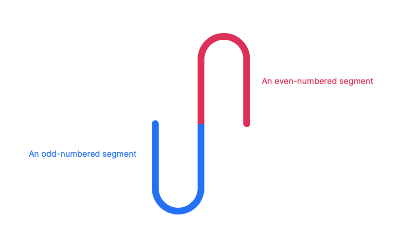
We still animate rotation.x of each box from 0 to 90 degrees, so the first mesh rotates to 90 degrees, the second one does the same 90 degrees plus its own 90 degrees rotation, the third does 90+90+90 degrees, etc.

A very easy and quite useful trick.

Animating the flaps

Back to the flaps. Flaps are made from translated geometry and added to the scene as children of the side meshes. We set their position.y property once and animate their rotation.x property on scroll.

function setGeometryHierarchy() {
    box.els.group.add(box.els.frontHalf.width.side, box.els.frontHalf.length.side, box.els.backHalf.width.side, box.els.backHalf.length.side);
    box.els.frontHalf.width.side.add(box.els.frontHalf.width.top, box.els.frontHalf.width.bottom);
    box.els.frontHalf.length.side.add(box.els.frontHalf.length.top, box.els.frontHalf.length.bottom);
    box.els.backHalf.width.side.add(box.els.backHalf.width.top, box.els.backHalf.width.bottom);
    box.els.backHalf.length.side.add(box.els.backHalf.length.top, box.els.backHalf.length.bottom);
}

function createBoxElements() {
    for (let halfIdx = 0; halfIdx < 2; halfIdx++) {
        for (let sideIdx = 0; sideIdx < 2; sideIdx++) {

            // ...

            const topGeometry = flapPlaneGeometry.clone();
            topGeometry.translate(0, .5 * flapHeight, 0);

            const bottomGeometry = flapPlaneGeometry.clone();
            bottomGeometry.translate(0, -.5 * flapHeight, 0);

            box.els[half][side].top.position.y = .5 * box.params.depth;
            box.els[half][side].bottom.position.y = -.5 * box.params.depth;
        }
    }
}

The animation of each flap has an individual timing and easing within the gsap.timeline so we store the flap angles separately.

let box = {
    // ...
    animated: {
        openingAngle: .02 * Math.PI,
        flapAngles: {
            backHalf: {
                width: {
                    top: 0,
                    bottom: 0
                },
                length: {
                    top: 0,
                    bottom: 0
                },
            },
            frontHalf: {
                width: {
                    top: 0,
                    bottom: 0
                },
                length: {
                    top: 0,
                    bottom: 0
                },
            }
        }
    }
}

function createFoldingAnimation() {
    gsap.timeline({
        scrollTrigger: {
            // ...
        },
        onUpdate: updatePanelsTransform
    })
        .to(box.animated, {
            duration: 1,
            openingAngle: .5 * Math.PI,
            ease: 'power1.inOut'
        })
        .to([ box.animated.flapAngles.backHalf.width, box.animated.flapAngles.frontHalf.width ], {
            duration: .6,
            bottom: .6 * Math.PI,
            ease: 'back.in(3)'
        }, .9)
        .to(box.animated.flapAngles.backHalf.length, {
            duration: .7,
            bottom: .5 * Math.PI,
            ease: 'back.in(2)'
        }, 1.1)
        .to(box.animated.flapAngles.frontHalf.length, {
            duration: .8,
            bottom: .49 * Math.PI,
            ease: 'back.in(3)'
        }, 1.4)
        .to([box.animated.flapAngles.backHalf.width, box.animated.flapAngles.frontHalf.width], {
            duration: .6,
            top: .6 * Math.PI,
            ease: 'back.in(3)'
        }, 1.4)
        .to(box.animated.flapAngles.backHalf.length, {
            duration: .7,
            top: .5 * Math.PI,
            ease: 'back.in(3)'
        }, 1.7)
        .to(box.animated.flapAngles.frontHalf.length, {
            duration: .9,
            top: .49 * Math.PI,
            ease: 'back.in(4)'
        }, 1.8)
}

function updatePanelsTransform() {

    // ... folding / unfolding

    box.els.frontHalf.width.top.rotation.x = -box.animated.flapAngles.frontHalf.width.top;
    box.els.frontHalf.length.top.rotation.x = -box.animated.flapAngles.frontHalf.length.top;
    box.els.frontHalf.width.bottom.rotation.x = box.animated.flapAngles.frontHalf.width.bottom;
    box.els.frontHalf.length.bottom.rotation.x = box.animated.flapAngles.frontHalf.length.bottom;

    box.els.backHalf.width.top.rotation.x = box.animated.flapAngles.backHalf.width.top;
    box.els.backHalf.length.top.rotation.x = box.animated.flapAngles.backHalf.length.top;
    box.els.backHalf.width.bottom.rotation.x = -box.animated.flapAngles.backHalf.width.bottom;
    box.els.backHalf.length.bottom.rotation.x = -box.animated.flapAngles.backHalf.length.bottom;
}

With all this, we finish the animation part! Let’s now work on the look of our box.

Lights and colors

This part is as simple as replacing multi-color wireframes with a single color MeshStandardMaterial and adding a few lights.

const ambientLight = new THREE.AmbientLight(0xffffff, .5);
scene.add(ambientLight);
lightHolder = new THREE.Group();
const topLight = new THREE.PointLight(0xffffff, .5);
topLight.position.set(-30, 300, 0);
lightHolder.add(topLight);
const sideLight = new THREE.PointLight(0xffffff, .7);
sideLight.position.set(50, 0, 150);
lightHolder.add(sideLight);
scene.add(lightHolder);

const material = new THREE.MeshStandardMaterial({
    color: new THREE.Color(0x9C8D7B),
    side: THREE.DoubleSide
});
box.els.group.traverse(c => {
    if (c.isMesh) c.material = material;
});

Tip: Object rotation effect with OrbitControls

OrbitControls make the camera orbit around the central point (left preview). To demonstrate a 3D object, it’s better to give users a feeling that they rotate the object itself, not the camera around it (right preview). To do so, we keep the lights position static relative to camera.

It can be done by wrapping lights in an additional lightHolder object. The pivot point of the parent object is (0, 0, 0). We also know that the camera rotates around (0, 0, 0). It means we can simply apply the camera’s rotation to the lightHolder to keep the lights static relative to the camera.

function render() {
    // ...
    lightHolder.quaternion.copy(camera.quaternion);
    renderer.render(scene, camera);
}

Layered panels

So far, our sides and flaps were done as a simple PlaneGeomery. Let’s replace it with “real” corrugated cardboard material ‐ two covers and a fluted layer between them.

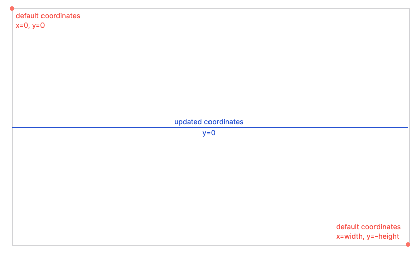
First step is replacing a single plane with 3 planes merged into one. To do so, we need to place 3 clones of PlaneGeometry one behind another and translate the front and back levels along the Z axis by half of the total cardboard thickness.

There’re many ways to move the layers, starting from the geometry.translate(0, 0, .5 * thickness) method we used to change the pivot point. But considering other transforms we’re about to apply to the cardboard geometry, we better go through the geometry.attributes.position array and add the offset to the z-coordinates directly:

fconst baseGeometry = new THREE.PlaneGeometry(
    params.width,
    params.height,
);

const geometriesToMerge = [
    getLayerGeometry(- .5 * params.thickness),
    getLayerGeometry(0),
    getLayerGeometry(.5 * params.thickness)
];

function getLayerGeometry(offset) {
    const layerGeometry = baseGeometry.clone();
    const positionAttr = layerGeometry.attributes.position;
    for (let i = 0; i < positionAttr.count; i++) {
        const x = positionAttr.getX(i);
        const y = positionAttr.getY(i)
        const z = positionAttr.getZ(i) + offset;
        positionAttr.setXYZ(i, x, y, z);
    }
    return layerGeometry;
}

For merging the geometries we use the mergeBufferGeometries method. It’s pretty straightforward, just don’t forget to import the BufferGeometryUtils module into your project.

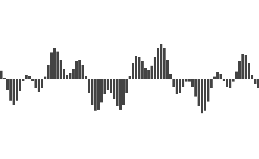
Wavy flute

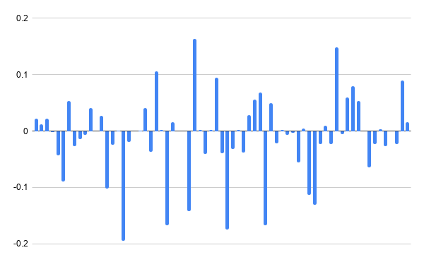
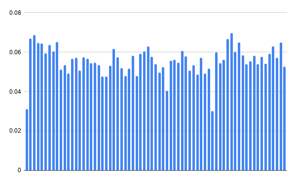
To turn a mid layer into the flute, we apply the sine wave to the plane. In fact, it’s the same z-coordinate offset, just calculated as Sine function of the x-attribute instead of a constant value.

function getLayerGeometry() {
    const baseGeometry = new THREE.PlaneGeometry(
        params.width,
        params.height,
        params.widthSegments,
        1
    );

    const offset = (v) => .5 * params.thickness * Math.sin(params.fluteFreq * v);
    const layerGeometry = baseGeometry.clone();
    const positionAttr = layerGeometry.attributes.position;
    for (let i = 0; i < positionAttr.count; i++) {
        const x = positionAttr.getX(i);
        const y = positionAttr.getY(i)
        const z = positionAttr.getZ(i) + offset(x);
        positionAttr.setXYZ(i, x, y, z);
    }
    layerGeometry.computeVertexNormals();

    return layerGeometry;
}

The z-offset is not the only change we need here. By default, PlaneGeometry is constructed from two triangles. As it has only one width segment and one height segment, there’re only corner vertices. To apply the sine(x) wave, we need enough vertices along the x axis – enough resolution, you can say.

Also, don’t forget to update the normals after changing the geometry. It doesn’t happen automatically.

I apply the wave with an amplitude equal to the cardboard thickness to the middle layer, and the same wave with a little amplitude to the front and back layers, just to give some texture to the box.

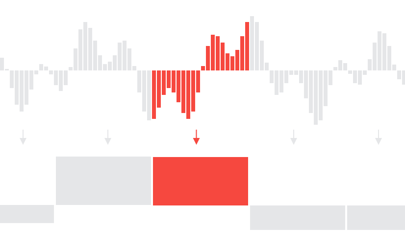
The surfaces and cuts look pretty cool. But we don’t want to see the wavy layer on the folding lines. At the same time, I want those lines to be visible before the folding happens:

To achieve this, we can “press” the cardboard on the selected edges of each panel.

We can do so by applying another modifier to the z-coordinate. This time it’s a power function of the x or y attribute (depending on the side we’re “pressing”).

function getLayerGeometry() {
    const baseGeometry = new THREE.PlaneGeometry(
        params.width,
        params.height,
        params.widthSegments,
        params.heightSegments // to apply folding we need sufficient number of segments on each side
    );

    const offset = (v) => .5 * params.thickness * Math.sin(params.fluteFreq * v);
    const layerGeometry = baseGeometry.clone();
    const positionAttr = layerGeometry.attributes.position;
    for (let i = 0; i < positionAttr.count; i++) {
        const x = positionAttr.getX(i);
        const y = positionAttr.getY(i)
        let z = positionAttr.getZ(i) + offset(x); // add wave
        z = applyFolds(x, y, z); // add folds
        positionAttr.setXYZ(i, x, y, z);
    }
    layerGeometry.computeVertexNormals();

    return layerGeometry;
}

function applyFolds(x, y, z) {
    const folds = [ params.topFold, params.rightFold, params.bottomFold, params.leftFold ];
    const size = [ params.width, params.height ];
    let modifier = (c, size) => (1. - Math.pow(c / (.5 * size), params.foldingPow));

    // top edge: Z -> 0 when y -> plane height,
    // bottom edge: Z -> 0 when y -> 0,
    // right edge: Z -> 0 when x -> plane width,
    // left edge: Z -> 0 when x -> 0

    if ((x > 0 && folds[1]) || (x < 0 && folds[3])) {
        z *= modifier(x, size[0]);
    }
    if ((y > 0 && folds[0]) || (y < 0 && folds[2])) {
        z *= modifier(y, size[1]);
    }
    return z;
}

The folding modifier is applied to all 4 edges of the box sides, to the bottom edges of the top flaps, and to the top edges of bottom flaps.

With this the box itself is finished.

There is room for optimization, and for some extra features, of course. For example, we can easily remove the flute level from the side panels as it’s never visible anyway. Let me also quickly describe how to add zooming buttons and a side image to our gorgeous box.

Zooming

The default behaviour of OrbitControls is zooming the scene by scroll. It means that our scroll-driven animation is in conflict with it, so we set orbit.enableZoom property to false.

We still can have zooming on the scene by changing the camera.zoom property. We can use the same GSAP animation as before, just note that animating the camera’s property doesn’t automatically update the camera’s projection. According to the documentation, updateProjectionMatrix() must be called after any change of the camera parameters so we have to call it on every frame of the transition:

// ...
// changing the zoomLevel variable with buttons

gsap.to(camera, {
    duration: .2,
    zoom: zoomLevel,
    onUpdate: () => {
        camera.updateProjectionMatrix();
    }
})

Side image

The image, or even a clickable link, can be added on the box side. It can be done with an additional plane mesh with a texture on it. It should be just moving together with the selected side of the box:

function updatePanelsTransform() {

   // ...

   // for copyright mesh to be placed on the front length side of the box
   copyright.position.copy(box.els.frontHalf.length.side.position);
   copyright.position.x += .5 * box.params.length - .5 * box.params.copyrightSize[0];
   copyright.position.y -= .5 * (box.params.depth - box.params.copyrightSize[1]);
   copyright.position.z += box.params.thickness;
}

As for the texture, we can import an image/video file, or use a canvas element we create programmatically. In the final demo I use a canvas with a transparent background, and two lines of text with an underline. Turning the canvas into a Three.js texture makes me able to map it on the plane:

function createCopyright() {
    
    // create canvas
    
    const canvas = document.createElement('canvas');
    canvas.width = box.params.copyrightSize[0] * 10;
    canvas.height = box.params.copyrightSize[1] * 10;
    const planeGeometry = new THREE.PlaneGeometry(box.params.copyrightSize[0], box.params.copyrightSize[1]);

    const ctx = canvas.getContext('2d');
    ctx.clearRect(0, 0, canvas.width, canvas.width);
    ctx.fillStyle = '#000000';
    ctx.font = '22px sans-serif';
    ctx.textAlign = 'end';
    ctx.fillText('ksenia-k.com', canvas.width - 30, 30);
    ctx.fillText('codepen.io/ksenia-k', canvas.width - 30, 70);

    ctx.lineWidth = 2;
    ctx.beginPath();
    ctx.moveTo(canvas.width - 160, 35);
    ctx.lineTo(canvas.width - 30, 35);
    ctx.stroke();
    ctx.beginPath();
    ctx.moveTo(canvas.width - 228, 77);
    ctx.lineTo(canvas.width - 30, 77);
    ctx.stroke();

    // create texture

    const texture = new THREE.CanvasTexture(canvas);

    // create mesh mapped with texture

    copyright = new THREE.Mesh(planeGeometry, new THREE.MeshBasicMaterial({
        map: texture,
        transparent: true,
        opacity: .5
    }));
    scene.add(copyright);
}

To make the text lines clickable, we do the following:

use Raycaster and mousemove event to track if the intersection between cursor ray and plane, change the cursor appearance if the mesh is hovered
if a click happened while the mesh is hovered, check the uv coordinate of intersection
if the uv coordinate is on the top half of the mesh (uv.y > .5) we open the first link, if uv coordinate is below .5, we go to the second link

The raycaster code is available in the full demo.

Thank you for scrolling this far!
Hope this tutorial can be useful for your Three.js projects ♡

April 20, 2020

Java Help: Cannot find symbol

I keep getting CircleInformation.java:13: error: cannot find symbol float circumference = 2 (PI radiusF)
^

April 11, 2020

I got stucked with the problem

Good evening to everyone. I have some troubles with a task I have to do. I need some assistance. Excuse me if I haven't searched thoroughly in the forum and there is a similar topic somewhere. Thank you!

Here's the issue:

You would take as input any analytic function of 1 independent variable and a closed
interval [a, b], on which the function is analytic. You have to find out the extrema(s) of
the function. Then you have to show whether the local extrema is maxima or minima.
Write a code which is going to find the solution of the above problem.

Examples:
f (x)=2 x
315 x
2
+36 x on [1, 5]
stationary points at x = 2 and x = 3 with end points at x = 1 and x = 5
extremas at x = 1 and x = 5
with x =1 is minimum (23) and x = 5 is maximum (55)

f (x)=sin (x) on [0, 2PI]
stationary points at x = PI/2 and x = -PI/2 with end points at x = 0 and x = 2PI
extremas at x = -PI/2 and x = PI/2
with x =-PI/2 is minimum (-1) and x = PI/2 is maximum (1)

examples of test cases:
Test case 1
(x, f(x)) = (0, 0), (1, -1), (2, 8), (3, 63), (4, 224), (-1, -1), (-2, 8), (-3, 63)
corner points, x = -3, 4
extremas, x = 0, -1, 1
maxima, x = 0
minima, x = -1, 1

Test case 2
(x, f(x)) = (0, 0), (1, 1), (2, 4), (3, 9), (4, 16), (-1, 1), (-2, 4), (-3, 9), (-4, 16)
corner points, x = -4, 4
extremas, x = 0, -4, 4
maxima, x = -4, 4
minima, x = 0

I'm really stuck and I don't know what exactly to do. I'll be very thankful if you give me some clues. Thank you one more time!

November 13, 2019

High-speed Light Trails in Three.js

Sometimes I tactically check Pinterest for inspiration and creative exploration. Although one could also call it chronic procrastinating, I always find captivating ideas for new WebGL projects. That’s the way I started my last water distortion effect.

Today’s tutorial is inspired by this alternative Akira poster. It has this beautiful traffic time lapse with infinite lights fading into the distance:

Based on this creative effect, I decided to re-create the poster vibe but make it real-time, infinite and also customizable. All in the comfort of your browser!

Through this article, we’ll use Three.js and learn how to:

instantiate geometries to create thousands (up to millions) of lights
make the lights move in an infinite loop
create frame rate independent animations to keep them consistent on all devices
and finally, create modular distortions to ease the creation of new distortions or changes to existing ones

It’s going to be an intermediate tutorial, and we’re going to skip over the basic Three.js setup. This tutorial assumes that you are familiar with the basics of Three.js.

Preparing the road and camera

To begin we’ll create a new Road class to encapsulate all the logic for our plane. It’s going to be a basic PlaneBufferGeometry with its height being the road’s length.

We want this plane to be flat on the ground and going further way. But Three.js creates a vertical plane at the center of the scene. We’ll rotate it on the x-axis to make it flat on the ground (y-axis).

We’ll also move it by half it’s length on the z-axis to position the start of the plane at the center of the scene.

We’re moving it on the z-axis because position translation happens after the rotation. While we set the plane’s length on the y-axis, after the rotation, the length is on the z-axis.

export class Road {
  constructor(webgl, options) {
    this.webgl = webgl;
    this.options = options;
  }
  init() {
    const options = this.options;
    const geometry = new THREE.PlaneBufferGeometry(
      options.width,
      options.length,
      20,
      200
    );
    const material = new THREE.ShaderMaterial({ 
       	fragmentShader, 
        vertexShader,
        uniforms: {
           uColor:  new THREE.Uniform(new THREE.Color(0x101012)) 
        }
    });
    const mesh = new THREE.Mesh(geometry, material);

    mesh.rotation.x = -Math.PI / 2;
    mesh.position.z = -options.length / 2;

    this.webgl.scene.add(mesh);
  }
}
const fragmentShader = `
    uniform vec3 uColor;
	void main(){
        gl_FragColor = vec4(uColor,1.);
    }
`;
const vertexShader = `
	void main(){
        vec3 transformed = position.xyz;
        gl_Position = projectionMatrix * modelViewMatrix * vec4(transformed.xyz, 1.);
	}
`

After rotating our plane, you’ll notice that it disappeared. It’s exactly lined up with the camera. We’ll have to move the camera a bit up the y-axis for a better shot of the plane.

We’ll also instantiate and initiate our plane and move it on the z-axis a bit to avoid any issues when we add the distortion later on:

class App {
	constructor(container, options){
		super(container);
		
        this.camera.position.z = -4;
        this.camera.position.y = 7;
        this.camera.position.x = 0;
        
        this.road = new Road(this, options);
	}
	init(){
        this.road.init();
        this.tick();
	}
}

If something is not working or looking right, zooming out the camera in the z-axis can help bring things into perspective.

Creating the lights

For the lights, we’ll create a CarLights class with a single tube geometry. We’ll use this single tube geometry as a base for all other lights.

All our tubes are going to have different lengths and radii. So, we’ll set the original tube’s length and radius to 1. Then, in the tube’s vertex shader, we’ll multiply the original length/radius by the desired values, resulting in the tube getting its final length and radius.

Three.js makes TubeGeometries using a Curve. To give it that length of 1, we’ll create the tube with a lineCurve3 with its endpoint at -1 in the z-axis.

import * as THREE from "three";
export class CarLights {
  constructor(webgl, options) {
    this.webgl = webgl;
    this.options = options;
  }
  init() {
      const options = this.options;
    let curve = new THREE.LineCurve3(
      new THREE.Vector3(0, 0, 0),
      new THREE.Vector3(0, 0, -1)
    );
    let baseGeometry = new THREE.TubeBufferGeometry(curve, 25, 1, 8, false);
    let material = new THREE.MeshBasicMaterial({ color: 0x545454 });
    let mesh = new THREE.Mesh(baseGeometry, material);
	
      this.mesh = mesh;
    this.webgl.scene.add(mesh);
  }
}

Instantiating the lights

Although some lights are longer or thicker than others, they all share the same geometry. Instead of creating a bunch of meshes for each light, and causing lots of draw calls, we can take advantage of instantiation.

Instantiation is the equivalent of telling WebGL “Hey buddy, render this SAME geometry X amount of times”. This process allows you to reduce the amount of draw calls to 1.

Although it’s the same result, rendering X objects, the process is very different. Let’s compare it with buying 50 chocolates at a store:

A draw call is the equivalent of going to the store, buying only one chocolate and then coming back. Then we repeat the process for all 50 chocolates. Paying for the chocolate (rendering) at the store is pretty fast, but going to the store and coming back (draw calls) takes a little bit of time. The more draw calls, the more trips to the store, the more time.

With instantiation, we’re going to the store and buying all 50 chocolates and coming back. You still have to go and come back from the store (draw call) one time. But you saved up those 49 extra trips.

A fun experiment to test this even further: Try to delete 50 different files from your computer, then try to delete just one file of equivalent size to all 50 combined. You’ll notice that even though it’s the same combined file size, the 50 files take more time to be deleted than the single file of equivalent size

Coming back to the code: to instantiate we’ll copy our tubeGeometry over to an InstancedBufferGeometry. Then we’ll tell it how many instances we’ll need. In our case, it’s going to be a number multiplied by 2 because we want two lights per “car”.

Next we’ll have to use that instanced geometry to create our mesh.

class CarLights {
    ...
	init(){
        ...
        let baseGeometry = new THREE.TubeBufferGeometry(curve, 25, 1, 8, false);
        let instanced = new THREE.InstancedBufferGeometry().copy(geometry);
        instanced.maxInstancedCount = options.nPairs * 2;
        ...
        // Use "Instanced" instead of "geometry"
        var mesh = new THREE.Mesh(instanced, material);
    }
}

Although it looks the same, Three.js now rendered 100 tubes in the same position. To move them to their respective positions we’ll use an InstancedBufferAttribute.

While a regular BufferAttribute describes the base shape, for example, it’s position, uvs, and normals, an InstanceBufferAttribute describes each instance of the base shape. In our case, each instance is going to have a different aOffset and a different radius/length aMetrics.

When it’s time each instance passes through the vertex shader. WebGL is going to give us the values corresponding to each instance. Then we can position them using those values.

We’ll loop over all the light pairs and calculate their XYZ position:

For the X-axis we’ll calculate the center of its lane. The width of the car, how separated the lights are, and a random offset.
For its Y-axis, we’ll push it up by its radius to make sure it’s on top of the road.
Finally, we’ll give it a random Z-offset based on the length of the road, putting some lights further away than others.

At the end of the loop, we’ll add the offset twice. Once per each light, with only the x-offset as a difference.

class CarLights {
    ...
    init(){
        ...
        let aOffset = [];

            let sectionWidth = options.roadWidth / options.roadSections;

            for (let i = 0; i < options.nPairs; i++) {
              let radius = 1.;
              // 1a. Get it's lane index
              // Instead of random, keep lights per lane consistent
              let section = i % 3;

              // 1b. Get its lane's centered position
              let sectionX =
                section * sectionWidth - options.roadWifth / 2 + sectionWidth / 2;
              let carWidth = 0.5 * sectionWidth;
              let offsetX = 0.5 * Math.random();

              let offsetY = radius * 1.3;

              aOffset.push(sectionX - carWidth / 2 + offsetX);
              aOffset.push(offsetY);
              aOffset.push(-offsetZ);

              aOffset.push(sectionX + carWidth / 2 + offsetX);
              aOffset.push(offsetY);
              aOffset.push(-offsetZ);
            }
        // Add the offset to the instanced geometry.
        instanced.addAttribute(
          "aOffset",
          new THREE.InstancedBufferAttribute(new Float32Array(aOffset), 3, false)
        );
        ...
    }
}

Now that we've added our aOffset attribute, let's go ahead and use it on a vertex shader like a regular bufferAttribute.

We'll replace our MeshBasicMaterial with a shaderMaterial and create a vertex shader where we'll add aOffset to the position:

class TailLights {
	init(){
		...
		const material = new THREE.ShaderMaterial({
			fragmentShader, 
            vertexShader,
            	uniforms: {
                    uColor: new THREE.Uniform(new THREE.Color('0xfafafa'))
                }
		})
		...
	}
}
const fragmentShader = `
uniform vec3 uColor;
  void main() {
      vec3 color = vec3(uColor);
      gl_FragColor = vec4(color,1.);
  }
`;

const vertexShader = `
attribute vec3 aOffset;
  void main() {
		vec3 transformed = position.xyz;

		// Keep them separated to make the next step easier!
	   transformed.z = transformed.z + aOffset.z;
        transformed.xy += aOffset.xy;
	
        vec4 mvPosition = modelViewMatrix * vec4(transformed,1.);
        gl_Position = projectionMatrix * mvPosition;
	}
`;

[https://codesandbox.io/s/infinite-lights-02-road-and-lights-coznb ]

Depending from where you look at the tubes, you'll notice that they might look odd. By default, Three.js' materials don't render the backside of faces side:THREE.FontSide.

While we could fix it by changing it to side: THREE.DoubleSide to render all sides, our tubes are going to be small and fast enough that you won't be able to notice the back faces aren't rendered. We can keep it like that for the sake of performance.

Giving tubes a different length and radius

Creating our tube with a length and radius of 1 was crucial for this section to work. Now we can set the radius and length of each instance only by multiplying on the vertex shader 1 * desiredRadius = desiredRadius.

Let's use the same loop to create a new instancedBufferAttribute called aMetrics. We'll store the length and radius of each instance here.

Remember that wee push to the array twice. One for each of the items in the pair.

class TailLights {
	...
	init(){
	...
	let aMetrics =[];
	for (let i = 0; i < totalLightsPairs; i++) {
     // We give it a minimum value to make sure the lights aren't too thin or short.
     // Give it some randomness but keep it over 0.1
      let radius = Math.random() * 0.1 + 0.1;
     // Give it some randomness but keep it over length *0.02
      let length =
        Math.random() * options.length * 0.08 + options.length * 0.02;
      
      aMetrics.push(radius);
      aMetrics.push(length);

      aMetrics.push(radius);
      aMetrics.push(length);
    }
    instanced.addAttribute(
      "aMetrics",
      new THREE.InstancedBufferAttribute(new Float32Array(aMetrics), 2, false)
    );
    ...
}

Note that we multiplied the position by aMetrics before adding any aOffset. This expands the tubes from their center, and then moves them to their position.

...
const vertexShader = `
attribute vec3 aOffset;
attribute vec2 aMetrics;
  void main() {
    vec3 transformed = position.xyz;

            float radius = aMetrics.r;
            float len = aMetrics.g;

            // 1. Set the radius and length
            transformed.xy *= radius; 
            transformed.z *= len;
		
    // 2. Then move the tubes
   transformed.z = transformed.z + aOffset.z;
   transformed.xy += aOffset.xy;

   vec4 mvPosition = modelViewMatrix * vec4(transformed,1.);
   gl_Position = projectionMatrix * mvPosition;
}
`;

Positioning the lights

We want to have two roads of lights coming from different directions. Let's create the second TailLights and move each to their respective position. To center them both, we'll move them by half the middle island's width and half the road's width.

We'll also give each light its color, and modify the material to use that instead:

class App {
    constructor(){
        this.leftLights  = new TailLights(this, options, 0xff102a);
        this.rightLights = new TailLights(this, options, 0xfafafa);
    }
	init(){
		...
		
        this.leftLights.init();
        this.leftLights.mesh.position.setX(
           -options.roadWidth / 2 - options.islandWidth / 2
        );
        this.rightLights.init();
        this.rightLights.mesh.position.setX(
           options.roadWidth / 2 + options.islandWidth / 2
        );

	}
}

class TailLights {
	constuctor(webgl, options, color){
		this.color = color;
		...
	}
        init(){
            ...
            const material = new THREE.ShaderMaterial({
                fragmentShader, 
                vertexShader,
                    uniforms: {
                        uColor: new THREE.Uniform(new THREE.Color(this.color))
                    }
            })
            ...
        }
}

Looking great! We can already start seeing how the project is coming together!

Moving and looping the lights

Because we created the tube's curve on the z-axis, moving the lights is only a matter of adding and subtracting from the z-axis. We'll use the elapsed time uTime because time is always moving and it's pretty consistent.

Let's begin with adding a uTime uniform and an update method. Then our App class can update the time on both our CarLights. And finally, we'll add time to the z-axis on the vertex shader:

class TailLights {
	init(){
		...
		cosnt material = new THREE.ShaderMaterial({
			fragmentShader, vertexShader,
            	uniforms: {
                    uColor: new THREE.Uniform(new THREE.Color(this.color)),
                    uTime: new THREE.Uniform(0),
                }
		})
		...
	}
        update(t){
            this.mesh.material.uniforms.uTime.value = t;
        }
}
const vertexShader = `
attribute vec3 aOffset;
attribute vec2 aMetrics;
  void main() {
    vec3 transformed = position.xyz;

    float radius = aMetrics.r;
    float len = aMetrics.g;
    transformed.xy *= radius; 
    transformed.z *= len;

            // 1. Add time, and it's position to make it move
            float zOffset = uTime + aOffset.z;
		
            // 2. Then place them in the correct position
            transformed.z += zOffset;

    transformed.xy += aOffset.xy;
	
    vec4 mvPosition = modelViewMatrix * vec4(transformed,1.);
    gl_Position = projectionMatrix * mvPosition;
	}
`;

class App {
  ...
  update(delta) {
    let time = this.clock.elapsedTime;
    this.leftLights.update(time);
    this.rightLights.update(time);
  }
}

It moves ultra-slow, but it moves!

Let's create a new uniform uSpeed and multiply it with uTime to make the animation go faster. Because each road has to go to a different side we'll also add it to the CarLights constructor to make it customizable.

class TailLights {
  constructor(webgl, options, color, speed) {
    ...
    this.speed = speed;
  }
	init(){
		...
		cosnt material = new THREE.ShaderMaterial({
			fragmentShader, vertexShader,
            	uniforms: {
                    uColor: new THREE.Uniform(new THREE.Color(this.color)),
                    uTime: new THREE.Uniform(0),
                    uSpeed: new THREE.Uniform(this.speed)
                }
		})
		...
	}
    ...
}
const vertexShader = `
attribute vec3 aOffset;
attribute vec2 aMetrics;
  void main() {
    vec3 transformed = position.xyz;

    // 1. Set the radius and length
    float radius = aMetrics.r;
    float len = aMetrics.g;
    transformed.xy *= radius; 
    transformed.z *= len;

    // 2. Add time, and it's position to make it move
        	float zOffset = uTime * uSpeed + aOffset.z;
			
    // 2. Then place them in the correct position
    transformed.z += zOffset;

    transformed.xy += aOffset.xy;
	
    vec4 mvPosition = modelViewMatrix * vec4(transformed,1.);
    gl_Position = projectionMatrix * mvPosition;
}
`;

Now that it's fast, let's make it loop.

We'll use the modulo operator mod to find the remainder of z-offset zOffset divided by the total road length uTravelLength. Getting only the remainder makes zOffset loop whenever it goes over uTravelLength.

Then, we'll subtract that from the z-axis and also add the length len to make it loop outside of the camera's view. And that's looping tubes!

Let's go ahead and add the uTravelLength uniform to our material:

class TailLights {
	init(){
		...
		cosnt material = new THREE.ShaderMaterial({
			fragmentShader, vertexShader,
            	uniforms: {
                    uColor: new THREE.Uniform(new THREE.Color(this.color)),
                    uTime: new THREE.Uniform(0),
                    uSpeed: new THREE.Uniform(this.speed)
                    uTime: new THREE.Uniform(0),
                }
		})
		...
	}
}

And let's modify the vertex shaders zOffset to make it loop:

const vertexShader = `
attribute vec3 aOffset;
attribute vec2 aMetrics;
uniform float uTime;
uniform float uSpeed;
uniform float uTravelLength;
  void main() {
    vec3 transformed = position.xyz;
    
    float radius = aMetrics.r;
    float len = aMetrics.g;
    transformed.xy *= radius; 
    transformed.z *= len;

        float zOffset = uTime * uSpeed + aOffset.z;
        // 1. Mod by uTravelLength to make it loop whenever it goes over
        // 2. Add len to make it loop a little bit later
        zOffset = len - mod(zOffset , uTravelLength);

   // Keep them separated to make the next step easier!
   transformed.z = transformed.z +zOffset ;
   transformed.xy += aOffset.xy;

   vec4 mvPosition = modelViewMatrix * vec4(transformed,1.);
   gl_Position = projectionMatrix * mvPosition;
}
`;

If you have a hawk's eye for faulty code, you'll noticed the loop isn't perfect. Behind the camera, the tubes go beyond the road's limits (push the camera back to see it in action). But for our use case, it does the job. Imperfect details outside of the camera don't matter.

Going faster and beyond

When holding left click we want our scene to go Speed Racer mode. Faster, and with a wider camera view.

Because the tube's speed is based on time, we'll add an extra offset to time whenever the left click is down. To make this transition extra smooth, we'll use linear interpolation (lerp) for the speedUp variable.

Note: We keep the timeOffset separate from the actual clock's time. Mutating the clock's time is never a good idea.

function lerp(current, target, speed = 0.1, limit = 0.001) {
  let change = (target - current) * speed;
  if (Math.abs(change) < limit) {
    change = target - current;
  }
  return change;
}

class App {
	constructor(){
		...
		this.speedUpTarget = 0.;
		this.speedUp = 0;
		this.timeOffset = 0;
		this.onMouseDown = this.onMouseDown.bind(this);
		this.onMouseUp = this.onMouseUp.bind(this);
	}
	init(){
		...
        this.container.addEventListener("mousedown", this.onMouseDown);
        this.container.addEventListener("mouseup", this.onMouseUp);
        this.container.addEventListener("mouseout", this.onMouseUp);
	}
  onMouseDown(ev) {
    this.speedUpTarget = 0.1;
  }
  onMouseUp(ev) {
    this.speedUpTarget = 0;
  }
  update(delta){
  	
      // Frame-dependent
    this.speedup += lerp(
      this.speedUp,
      this.speedUpTarget,
        // 10% each frame
      0.1,
      0.00001
    );
      // Also frame-dependent
    this.timeOffset += this.speedUp;
      
      
    let time = this.clock.elapsedTime + this.timeOffset;
    ...
    
  }
}

This is a totally functional and valid animation for our super speed mode; after all, it works. But it'll work differently depending on your Frames Per Second (FPS).

Frame rate independent speed up

The issue with the code above is that every frame we are adding a flat amount to the speed. This animation's speed depends on the frame rate.

It means if your frame rate suddenly becomes lower, or your frame rate was low to begin with, the animation is going to become slower as well. And if your frame rate is higher, the animation is going to speed up.

Resulting in the animations running faster or slower or depending on how many frames per second your computer can achieve, a frame rate dependent animation that takes 2 seconds at 30ps, takes 1 second at 60fps.

Our goal is to animate things using real-time. For all computers, the animations should always take X amount of seconds.

Looking back at our code, we have two animations that are frame rate dependent:

the speedUp's linear interpolation by 0.1 each frame
adding speedUp to timeOffset each frame

Adding speedUp to timeOffset is a linear process; it only depends on the speedup variable. So, we can make it frame rate independent by multiplying it by how many seconds have passed since the last frame (delta).

This one-line change makes the addition one this.speedUp per second. You might need to bump up the speed since the change makes the addition happen through a whole second.

class App {
	update(delta){
		...
         this.timeOffset += this.speedup * delta;		
		...
	} 
 }

Making the speedUp linear interpolation frame rate independent requires a little bit more math.

In the previous case, adding this.speedUp was a linear process, only dependent on the speedUp value. To make it frame rate independent we used another linear process: multiplying it by delta.

In the case of linear interpolation (lerp), we are trying to move towards the target 10% of the difference each time. This is not a linear process but an exponential process. To make it frame rate independent, we need another exponential process that involves delta.

We'll use the functions found in this article about making lerp frame rate independent.

Instead of moving towards the target 10% each frame, we'll move towards the target based on an exponential function based on time delta instead.

let coefficient = 0.1;
let lerpT = Math.exp(-coefficient * delta); 
this.speedup += lerp(
      this.speedup,
      this.speedupTarget,
      lerpT,
      0.00001
    );

This modification completely changes how our coefficient works. Now, a coefficient of 1.0 moves halfway to the target each second.

If we want to use our old coefficients 0.1 that we know already works fine for 60fps, we can convert the old coefficient into the new ones like this:

let coefficient = -60*Math.log2(1 - 0.1);

Plot twist: Math is actually hard. Although there are some great links out there explaining how all the math makes sense, some of it still flies over my head. If you know more about the theory of why all of this works. Feel free to reach out or type it in the comments. I would love to have a chat!

Repeat the process for the Camera's Field Of View camera.fov. And we also get a frame rate independent animation for the fov. We'll reuse the same lerpT to make it easier.

class App {
	constructor(){
		...
        this.fovTarget = 90;
        ...
	}
  onMouseDown(ev) {
    this.fovTarget = 140;
    ...
  }
  onMouseUp(ev) {
    this.fovTarget = 90;
     ...
  }
  update(delta){
      ...
    let fovChange = lerp(this.camera.fov, this.fovTarget, lerpT );
    if (fovChange !== 0) {
      this.camera.fov += fovChange * delta * 6.;
      this.camera.updateProjectionMatrix();
    }
    ...
    
  }
}

Note: Don't forget to update its transformation matrix after you are done with the changes or it won't update in the GPU.

Modularized distortion

The distortion of each object happens on the vertex shader. And as you can see, all objects share the same distortion. But GLSL doesn't have a module system unless you add something like glslify. If you want to reuse and swap pieces of GLSL code, you have to create that system yourself with JavaScript.

Alternatively, if you have only one or two shaders that need distortion, you can always hard code the distortion GLSL code on each mesh's shader. Then, update each one every time you make a change to the distortion. But try to keep track of updating more than two shaders and you start going insane quickly.

In my case, I chose to keep my sanity and create my own little system. This way I could create multiple distortions and play around with the values for the different demos.

Each distortion is an object with three main properties:

distortion_uniforms: The uniforms this distortion is going to need. Each mesh takes care of adding these into their material.
distortion_chunk: The GLSL code that exposes getDistortion function for the shaders that implement it. getDistortion receives a normalized value progress indicating how far into the road is the point. It returns the distortion of that specific position.
(Optional) getJS: The GLSL code ported to JavaScript. This is useful for creating JS interactions following the curve. Like the camera rotating to face the road as we move along.

const distortion_uniforms = {
  uDistortionX: new THREE.Uniform(new THREE.Vector2(80, 3)),
  uDistortionY: new THREE.Uniform(new THREE.Vector2(-40, 2.5))
};

const distortion_vertex = `
#define PI 3.14159265358979
  uniform vec2 uDistortionX;
  uniform vec2 uDistortionY;

    float nsin(float val){
    return sin(val) * 0.5+0.5;
    }
  vec3 getDistortion(float progress){
        progress = clamp(progress, 0.,1.);
        float xAmp = uDistortionX.r;
        float xFreq = uDistortionX.g;
        float yAmp = uDistortionY.r;
        float yFreq = uDistortionY.g;
        return vec3( 
            xAmp * nsin(progress* PI * xFreq   - PI / 2. ) ,
            yAmp * nsin(progress * PI *yFreq - PI / 2.  ) ,
            0.
        );
    }
`;

const myCustomDistortion = {
    uniforms: distortion_uniforms,
    getDistortion: distortion_vertex,
}

Then, you pass the distortion object as a property in the options given when instantiating the main App class like so:

const myApp = new App(
	container, 
	{
        ... // Bunch of other options
		distortion: myCustomDistortion,
        ...
    }
)
...

From here each object can take the distortion from the options and use it as it needs.

Both, the CarLights and Road classes are going to add distortion.uniforms to their material and modify their shader using Three.js' onBeforeCompile:

const material = new THREE.ShaderMaterial({
	...
	uniforms: Object.assign(
		{...}, // The original uniforms of this object
		options.uniforms
	)
})

material.onBeforeCompile = shader => {
  shader.vertexShader = shader.vertexShader.replace(
    "#include ",
    options.distortion.getDistortion
  );
};

Before Three.js sends our shaders to webGL it checks it's custom GLSL to inject any ShaderChunks your shader needs. onBeforeCompile is a function that happens before Three.js compiles your shader into valid GLSL code. Making it easy to extend any built-in materials.

In our case, we'll use onBeforeCompile to inject our distortion's code. Only to avoid the hassle of injecting it another way.

As it stands now, we aren't injecting any code. We first need to add #include <getDistortion_vertex> to our shaders.

In our CarLights vertex shader we need to map its z-position as its distortion progress. And we'll add the distortion after all other math, right at the end:

// Car Lights Vertex shader
const vertexShader = `
attribute vec3 aOffset;
attribute vec2 aMetrics;
uniform float uTime;
uniform float uSpeed;
uniform float uTravelLength;
#include 
  void main() {
	...
        

		// Map z-position to progress: A range of 0 to 1.
        float progress = abs(transformed.z / uTravelLength);
        transformed.xyz += getDistortion(progress);

	
        vec4 mvPosition = modelViewMatrix * vec4(transformed,1.);
        gl_Position = projectionMatrix * mvPosition;
	}
`;

In our Road class, although we see it flat going towards negative-z because we rotated it, this mesh rotation happens after the vertex shader. In the eyes of our shader, our plane is still vertical y-axis and placed in the center of the scene.

To get the correct distortion, we need to map the y-axis as progress. First, we'll un-center it uTravelLength /2., and then we'll normalize it.

Also, instead of adding the y-distortion to the y-axis, we'll add it to the z-axis instead. Remember, in the vertex shader, the rotation hasn't happened yet.

// Road Vertex shader
const vertexShader = `
uniform float uTravelLength;
#include 
	void main(){
        vec3 transformed = position.xyz;
        
	// Normalize progress to a range of 0 to 1
    float progress = (transformed.y + uTravelLength / 2.) / uTravelLength;
    vec3 distortion  = getDistortion(progress);
    transformed.x += distortion.x;
	// z-axis is becomes the y-axis after mesh rotation. 
    transformed.z += distortion.y;
    gl_Position = projectionMatrix * modelViewMatrix * vec4(transformed.xyz, 1.);
	}
`;

An there you have the final result for this tutorial!

Finishing touches

There are a few ways you can expand and better sell the effect of an infinite road in the middle of the night. Like creating more interesting curves and fading the objects into the background with some fog effect to make the lights seem like they are glowing.

Final Thoughts

I find that re-creating things from outside of the web and simply doing some creative coding, opens me up to a wider range of interesting ideas.

In this tutorial, we learned how to instantiate geometries, create frame rate independent animations and modulized distortions. And we brought it all together to re-create and put some motion into this awesome poster!

Hopefully, you've also liked working through this tutorial! Let me know what you think in the comments and feel free to reach out to me!

High-speed Light Trails in Three.js was written by Daniel Velasquez and published on Codrops.

November 12, 2019

Making an Audio Waveform Visualizer with Vanilla JavaScript

As a UI designer, I’m constantly reminded of the value of knowing how to code. I pride myself on thinking of the developers on my team while designing user interfaces. But sometimes, I step on a technical landmine.

A few years ago, as the design director of wsj.com, I was helping to re-design the Wall Street Journal’s podcast directory. One of the designers on the project was working on the podcast player, and I came upon Megaphone’s embedded player.

I previously worked at SoundCloud and knew that these kinds of visualizations were useful for users who skip through audio. I wondered if we could achieve a similar look for the player on the Wall Street Journal’s site.

The answer from engineering: definitely not. Given timelines and restraints, it wasn’t a possibility for that project. We eventually shipped the redesigned pages with a much simpler podcast player.

But I was hooked on the problem. Over nights and weekends, I hacked away trying to achieve this
effect. I learned a lot about how audio works on the web, and ultimately was able to achieve the look with less than 100 lines of JavaScript!

It turns out that this example is a perfect way to get acquainted with the Web Audio API, and how to visualize audio data using the Canvas API.

But first, a lesson in how digital audio works

In the real, analog world, sound is a wave. As sound travels from a source (like a speaker) to your ears, it compresses and decompresses air in a pattern that your ears and brain hear as music, or speech, or a dog’s bark, etc. etc.

An analog sound wave is a smooth, continuous function.

But in a computer’s world of electronic signals, sound isn’t a wave. To turn a smooth, continuous wave into data that it can store, computers do something called sampling. Sampling means measuring the sound waves hitting a microphone thousands of times every second, then storing those data points. When playing back audio, your computer reverses the process: it recreates the sound, one tiny split-second of audio at a time.

A digital sound file is made up of tiny slices of the original audio, roughly re-creating the smooth continuous wave.

The number of data points in a sound file depends on its sample rate. You might have seen this number before; the typical sample rate for mp3 files is 44.1 kHz. This means that, for every second of audio, there are 44,100 individual data points. For stereo files, there are 88,200 every second — 44,100 for the left channel, and 44,100 for the right. That means a 30-minute podcast has 158,760,000 individual data points describing the audio!

How can a web page read an mp3?

Over the past nine years, the W3C (the folks who help maintain web standards) have developed the Web Audio API to help web developers work with audio. The Web Audio API is a very deep topic; we’ll hardly crack the surface in this essay. But it all starts with something called the AudioContext.

Think of the AudioContext like a sandbox for working with audio. We can initialize it with a few lines of JavaScript:

// Set up audio context
window.AudioContext = window.AudioContext || window.webkitAudioContext;
const audioContext = new AudioContext();
let currentBuffer = null;

The first line after the comment is a necessary because Safari has implemented AudioContext as webkitAudioContext.

Next, we need to give our new audioContext the mp3 file we’d like to visualize. Let’s fetch it using… fetch()!

const visualizeAudio = url => {
  fetch(url)
    .then(response => response.arrayBuffer())
    .then(arrayBuffer => audioContext.decodeAudioData(arrayBuffer))
    .then(audioBuffer => visualize(audioBuffer));
};

This function takes a URL, fetches it, then transforms the Response object a few times.

First, it calls the arrayBuffer() method, which returns — you guessed it — an ArrayBuffer! An ArrayBuffer is just a container for binary data; it’s an efficient way to move lots of data around in JavaScript.
We then send the ArrayBuffer to our audioContext via the decodeAudioData() method. decodeAudioData() takes an ArrayBuffer and returns an AudioBuffer, which is a specialized ArrayBuffer for reading audio data. Did you know that browsers came with all these convenient objects? I definitely did not when I started this project.
Finally, we send our AudioBuffer off to be visualized.

Filtering the data

To visualize our AudioBuffer, we need to reduce the amount of data we’re working with. Like I mentioned before, we started off with millions of data points, but we’ll have far fewer in our final visualization.

First, let’s limit the channels we are working with. A channel represents the audio sent to an individual speaker. In stereo sound, there are two channels; in 5.1 surround sound, there are six. AudioBuffer has a built-in method to do this: getChannelData(). Call audioBuffer.getChannelData(0), and we’ll be left with one channel’s worth of data.

Next, the hard part: loop through the channel’s data, and select a smaller set of data points. There are a few ways we could go about this. Let’s say I want my final visualization to have 70 bars; I can divide up the audio data into 70 equal parts, and look at a data point from each one.

const filterData = audioBuffer => {
  const rawData = audioBuffer.getChannelData(0); // We only need to work with one channel of data
  const samples = 70; // Number of samples we want to have in our final data set
  const blockSize = Math.floor(rawData.length / samples); // Number of samples in each subdivision
  const filteredData = [];
  for (let i = 0; i < samples; i++) {
    filteredData.push(rawData[i * blockSize]); 
  }
  return filteredData;
}

This was the first approach I took. To get an idea of what the filtered data looks like, I put the result into a spreadsheet and charted it.

The output caught me off guard! It doesn’t look like the visualization we’re emulating at all. There are lots of data points that are close to, or at zero. But that makes a lot of sense: in a podcast, there is a lot of silence between words and sentences. By only looking at the first sample in each of our blocks, it’s highly likely that we’ll catch a very quiet moment.

Let’s modify the algorithm to find the average of the samples. And while we’re at it, we should take the absolute value of our data, so that it’s all positive.

const filterData = audioBuffer => {
  const rawData = audioBuffer.getChannelData(0); // We only need to work with one channel of data
  const samples = 70; // Number of samples we want to have in our final data set
  const blockSize = Math.floor(rawData.length / samples); // the number of samples in each subdivision
  const filteredData = [];
  for (let i = 0; i < samples; i++) {
    let blockStart = blockSize * i; // the location of the first sample in the block
    let sum = 0;
    for (let j = 0; j < blockSize; j++) {
      sum = sum + Math.abs(rawData[blockStart + j]) // find the sum of all the samples in the block
    }
    filteredData.push(sum / blockSize); // divide the sum by the block size to get the average
  }
  return filteredData;
}

Let’s see what that data looks like.

This is great. There’s only one thing left to do: because we have so much silence in the audio file, the resulting averages of the data points are very small. To make sure this visualization works for all audio files, we need to normalize the data; that is, change the scale of the data so that the loudest samples measure as 1.

const normalizeData = filteredData => {
  const multiplier = Math.pow(Math.max(...filteredData), -1);
  return filteredData.map(n => n * multiplier);
}

This function finds the largest data point in the array with Math.max(), takes its inverse with Math.pow(n, -1), and multiplies each value in the array by that number. This guarantees that the largest data point will be set to 1, and the rest of the data will scale proportionally.

Now that we have the right data, let’s write the function that will visualize it.

Visualizing the data

To create the visualization, we’ll be using the JavaScript Canvas API. This API draws graphics into an HTML <canvas> element. The first step to using the Canvas API is similar to the Web Audio API.

const draw = normalizedData => {
  // Set up the canvas
  const canvas = document.querySelector("canvas");
  const dpr = window.devicePixelRatio || 1;
  const padding = 20;
  canvas.width = canvas.offsetWidth * dpr;
  canvas.height = (canvas.offsetHeight + padding * 2) * dpr;
  const ctx = canvas.getContext("2d");
  ctx.scale(dpr, dpr);
  ctx.translate(0, canvas.offsetHeight / 2 + padding); // Set Y = 0 to be in the middle of the canvas
};

This code finds the <canvas> element on the page, and checks the browser’s pixel ratio (essentially the screen’s resolution) to make sure our graphic will be drawn at the right size. We then get the context of the canvas (its individual set of methods and values). We calculate the pixel dimensions pf the canvas, factoring in the pixel ratio and adding in some padding. Lastly, we change the coordinates system of the <canvas>; by default, (0,0) is in the top-left of the box, but we can save ourselves a lot of math by setting (0, 0) to be in the middle of the left edge.

Now let’s draw some lines! First, we’ll create a function that will draw an individual segment.

const drawLineSegment = (ctx, x, y, width, isEven) => {
  ctx.lineWidth = 1; // how thick the line is
  ctx.strokeStyle = "#fff"; // what color our line is
  ctx.beginPath();
  y = isEven ? y : -y;
  ctx.moveTo(x, 0);
  ctx.lineTo(x, y);
  ctx.arc(x + width / 2, y, width / 2, Math.PI, 0, isEven);
  ctx.lineTo(x + width, 0);
  ctx.stroke();
};

The Canvas API uses an concept called “turtle graphics.” Imagine that the code is a set of instructions being given to a turtle with a marker. In basic terms, the drawLineSegment() function works as follows:

Start at the center line, x = 0.
Draw a vertical line. Make the height of the line relative to the data.
Draw a half-circle the width of the segment.
Draw a vertical line back to the center line.

Most of the commands are straightforward: ctx.moveTo() and ctx.lineTo() move the turtle to the specified coordinate, without drawing or while drawing, respectively.

Line 5, y = isEven ? -y : y, tells our turtle whether to draw down or up from the center line. The segments alternate between being above and below the center line so that they form a smooth wave. In the world of the Canvas API, negative y values are further up than positive ones. This is a bit counter-intuitive, so keep it in mind as a possible source of bugs.

On line 8, we draw a half-circle. ctx.arc() takes six parameters:

The x and y coordinates of the center of the circle
The radius of the circle
The place in the circle to start drawing (Math.PI or π is the location, in radians, of 9 o’clock)
The place in the circle to finish drawing (0 in radians represents 3 o’clock)
A boolean value telling our turtle to draw either counterclockwise (if true) or clockwise (if false). Using isEven in this last argument means that we’ll draw the top half of a circle — clockwise from 9 o’clock to 3 clock — for even-numbered segments, and the bottom half for odd-numbered segments.

OK, back to the draw() function.

const draw = normalizedData => {
  // Set up the canvas
  const canvas = document.querySelector("canvas");
  const dpr = window.devicePixelRatio || 1;
  const padding = 20;
  canvas.width = canvas.offsetWidth * dpr;
  canvas.height = (canvas.offsetHeight + padding * 2) * dpr;
  const ctx = canvas.getContext("2d");
  ctx.scale(dpr, dpr);
  ctx.translate(0, canvas.offsetHeight / 2 + padding); // Set Y = 0 to be in the middle of the canvas

  // draw the line segments
  const width = canvas.offsetWidth / normalizedData.length;
  for (let i = 0; i < normalizedData.length; i++) {
    const x = width * i;
    let height = normalizedData[i] * canvas.offsetHeight - padding;
    if (height < 0) {
        height = 0;
    } else if (height > canvas.offsetHeight / 2) {
        height = height > canvas.offsetHeight / 2;
    }
    drawLineSegment(ctx, x, height, width, (i + 1) % 2);
  }
};

After our previous setup code, we need to calculate the pixel width of each line segment. This is the canvas’s on-screen width, divided by the number of segments we’d like to display.

Then, a for-loop goes through each entry in the array, and draws a line segment using the function we defined earlier. We set the x value to the current iteration’s index, times the segment width. height, the desired height of the segment, comes from multiplying our normalized data by the canvas’s height, minus the padding we set earlier. We check a few cases: subtracting the padding might have pushed height into the negative, so we re-set that to zero. If the height of the segment will result in a line being drawn off the top of the canvas, we re-set the height to a maximum value.

We pass in the segment width, and for the isEven value, we use a neat trick: (i + 1) % 2 means “find the reminder of i + 1 divided by 2.” We check i + 1 because our counter starts at 0. If i + 1 is even, its remainder will be zero (or false). If i is odd, its remainder will be 1 or true.

And that’s all she wrote. Let’s put it all together. Here’s the whole script, in all its glory.

See the Pen
Audio waveform visualizer by Matthew Ström (@matthewstrom)
on CodePen.

In the drawAudio() function, we’ve added a few functions to the final call: draw(normalizeData(filterData(audioBuffer))). This chain filters, normalizes, and finally draws the audio we get back from the server.

If everything has gone according to plan, your page should look like this:

Notes on performance

Even with optimizations, this script is still likely running hundreds of thousands of operations in the browser. Depending on the browser’s implementation, this can take many seconds to finish, and will have a negative impact on other computations happening on the page. It also downloads the whole audio file before drawing the visualization, which consumes a lot of data. There are a few ways that we could improve the script to resolve these issues:

Analyze the audio on the server side. Since audio files don’t change often, we can take advantage of server-side computing resources to filter and normalize the data. Then, we only have to transmit the smaller data set; no need to download the mp3 to draw the visualization!
Only draw the visualization when a user needs it. No matter how we analyze the audio, it makes sense to defer the process until well after page load. We could either wait until the element is in view using an intersection observer, or delay even longer until a user interacts with the podcast player.
Progressive enhancement. While exploring Megaphone’s podcast player, I discovered that their visualization is just a facade — it’s the same waveform for every podcast. This could serve as a great default to our (vastly superior) design. Using the principles of progressive enhancement, we could load a default image as a placeholder. Then, we can check to see if it makes sense to load the real waveform before initiating our script. If the user has JavaScript disabled, their browser doesn’t support the Web Audio API, or they have the save-data header set, nothing is broken.

I’d love to hear any thoughts y’all have on optimization, too.

Some closing thoughts

This is a very, very impractical way of visualizing audio. It runs on the client side, processing millions of data points into a fairly straightforward visualization.

But it’s cool! I learned a lot in writing this code, and even more in writing this article. I refactored a lot of the original project and trimmed the whole thing in half. Projects like this might not ever go on to see a production codebase, but they are unique opportunities to develop new skills and a deeper understanding of some of the neat APIs modern browsers support.

I hope this was a helpful tutorial. If you have ideas of how to improve it, or any cool variations on the theme, please reach out! I’m @ilikescience on Twitter.

The post Making an Audio Waveform Visualizer with Vanilla JavaScript appeared first on CSS-Tricks.

January 17, 2019

Interactive Particles with Three.js

This tutorial is going to demonstrate how to draw a large number of particles with Three.js and an efficient way to make them react to mouse and touch input using shaders and an off-screen texture.

Attention: You will need an intermediate level of experience with Three.js. We will omit some parts of the code for brevity and assume you already know how to set up a Three.js scene and how to import your shaders — in this demo we are using glslify.

Instanced Geometry

The particles are created based on the pixels of an image. Our image’s dimensions are 320×180, or 57,600 pixels.

However, we don’t need to create one geometry for each particle. We can create only a single one and render it 57,600 times with different parameters. This is called geometry instancing. With Three.js we use InstancedBufferGeometry to define the geometry, BufferAttribute for attributes which remain the same for every instance and InstancedBufferAttribute for attributes which can vary between instances (i.e. colour, size).

The geometry of our particles is a simple quad, formed by 4 vertices and 2 triangles.


const geometry = new THREE.InstancedBufferGeometry();

// positions
const positions = new THREE.BufferAttribute(new Float32Array(4 * 3), 3);
positions.setXYZ(0, -0.5, 0.5, 0.0);
positions.setXYZ(1, 0.5, 0.5, 0.0);
positions.setXYZ(2, -0.5, -0.5, 0.0);
positions.setXYZ(3, 0.5, -0.5, 0.0);
geometry.addAttribute('position', positions);

// uvs
const uvs = new THREE.BufferAttribute(new Float32Array(4 * 2), 2);
uvs.setXYZ(0, 0.0, 0.0);
uvs.setXYZ(1, 1.0, 0.0);
uvs.setXYZ(2, 0.0, 1.0);
uvs.setXYZ(3, 1.0, 1.0);
geometry.addAttribute('uv', uvs);

// index
geometry.setIndex(new THREE.BufferAttribute(new Uint16Array([ 0, 2, 1, 2, 3, 1 ]), 1));

Next, we loop through the pixels of the image and assign our instanced attributes. Since the word position is already taken, we use the word offset to store the position of each instance. The offset will be the x,y of each pixel in the image. We also want to store the particle index and a random angle which will be used later for animation.


const indices = new Uint16Array(this.numPoints);
const offsets = new Float32Array(this.numPoints * 3);
const angles = new Float32Array(this.numPoints);

for (let i = 0; i < this.numPoints; i++) {
	offsets[i * 3 + 0] = i % this.width;
	offsets[i * 3 + 1] = Math.floor(i / this.width);

	indices[i] = i;

	angles[i] = Math.random() * Math.PI;
}

geometry.addAttribute('pindex', new THREE.InstancedBufferAttribute(indices, 1, false));
geometry.addAttribute('offset', new THREE.InstancedBufferAttribute(offsets, 3, false));
geometry.addAttribute('angle', new THREE.InstancedBufferAttribute(angles, 1, false));

Particle Material

The material is a RawShaderMaterial with custom shaders particle.vert and particle.frag.

The uniforms are described as follows:

uTime: elapsed time, updated every frame
uRandom: factor of randomness used to displace the particles in x,y
uDepth: maximum oscillation of the particles in z
uSize: base size of the particles
uTexture: image texture
uTextureSize: dimensions of the texture
uTouch: touch texture


const uniforms = {
	uTime: { value: 0 },
	uRandom: { value: 1.0 },
	uDepth: { value: 2.0 },
	uSize: { value: 0.0 },
	uTextureSize: { value: new THREE.Vector2(this.width, this.height) },
	uTexture: { value: this.texture },
	uTouch: { value: null }
};

const material = new THREE.RawShaderMaterial({
	uniforms,
	vertexShader: glslify(require('../../../shaders/particle.vert')),
	fragmentShader: glslify(require('../../../shaders/particle.frag')),
	depthTest: false,
	transparent: true
});

A simple vertex shader would output the position of the particles according to their offset attribute directly. To make things more interesting, we displace the particles using random and noise. And the same goes for particles’ sizes.


// particle.vert

void main() {
	// displacement
	vec3 displaced = offset;
	// randomise
	displaced.xy += vec2(random(pindex) - 0.5, random(offset.x + pindex) - 0.5) * uRandom;
	float rndz = (random(pindex) + snoise_1_2(vec2(pindex * 0.1, uTime * 0.1)));
	displaced.z += rndz * (random(pindex) * 2.0 * uDepth);

	// particle size
	float psize = (snoise_1_2(vec2(uTime, pindex) * 0.5) + 2.0);
	psize *= max(grey, 0.2);
	psize *= uSize;

	// (...)
}

The fragment shader samples the RGB colour from the original image and converts it to greyscale using the luminosity method (0.21 R + 0.72 G + 0.07 B).

The alpha channel is determined by the linear distance to the centre of the UV, which essentially creates a circle. The border of the circle can be blurred out using smoothstep.


// particle.frag

void main() {
	// pixel color
	vec4 colA = texture2D(uTexture, puv);

	// greyscale
	float grey = colA.r * 0.21 + colA.g * 0.71 + colA.b * 0.07;
	vec4 colB = vec4(grey, grey, grey, 1.0);

	// circle
	float border = 0.3;
	float radius = 0.5;
	float dist = radius - distance(uv, vec2(0.5));
	float t = smoothstep(0.0, border, dist);

	// final color
	color = colB;
	color.a = t;

	// (...)
}

Optimisation

In our demo we set the size of the particles according to their brightness, which means dark particles are almost invisible. This makes room for some optimisation. When looping through the pixels of the image, we can discard the ones which are too dark. This reduces the number of particles and improves performance.

The optimisation starts before we create our InstancedBufferGeometry. We create a temporary canvas, draw the image onto it and call getImageData() to retrieve an array of colours [R, G, B, A, R, G, B … ]. We then define a threshold — hex #22 or decimal 34 — and test it against the red channel. The red channel is an arbitrary choice, we could also use green or blue, or even an average of all three channels, but the red channel is simple to use.


// discard pixels darker than threshold #22
if (discard) {
	numVisible = 0;
	threshold = 34;

	const img = this.texture.image;
	const canvas = document.createElement('canvas');
	const ctx = canvas.getContext('2d');

	canvas.width = this.width;
	canvas.height = this.height;
	ctx.scale(1, -1); // flip y
	ctx.drawImage(img, 0, 0, this.width, this.height * -1);

	const imgData = ctx.getImageData(0, 0, canvas.width, canvas.height);
	originalColors = Float32Array.from(imgData.data);

	for (let i = 0; i < this.numPoints; i++) {
		if (originalColors[i * 4 + 0] > threshold) numVisible++;
	}
}

We also need to update the loop where we define offset, angle and pindex to take the threshold into account.


for (let i = 0, j = 0; i < this.numPoints; i++) {
	if (originalColors[i * 4 + 0] <= threshold) continue;

	offsets[j * 3 + 0] = i % this.width;
	offsets[j * 3 + 1] = Math.floor(i / this.width);

	indices[j] = i;

	angles[j] = Math.random() * Math.PI;

	j++;
}

Interactivity

Considerations

There are many different ways of introducing interaction with the particles. For example, we could give each particle a velocity attribute and update it on every frame based on its proximity to the cursor. This is a classic technique and it works very well, but it might be a bit too heavy if we have to loop through tens of thousands of particles.

A more efficient way would be to do it in the shader. We could pass the cursor’s position as a uniform and displace the particles based on their distance from it. While this would perform a lot faster, the result could be quite dry. The particles would go to a given position, but they wouldn’t ease in or out of it.

Chosen Approach

The technique we chose in our demo was to draw the cursor position onto a texture. The advantage is that we can keep a history of cursor positions and create a trail. We can also apply an easing function to the radius of that trail, making it grow and shrink smoothly. Everything would happen in the shader, running in parallel for all the particles.

In order to get the cursor’s position we use a Raycaster and a simple PlaneBufferGeometry the same size of our main geometry. The plane is invisible, but interactive.

Interactivity in Three.js is a topic on its own. Please see this example for reference.

When there is an intersection between the cursor and the plane, we can use the UV coordinates in the intersection data to retrieve the cursor’s position. The positions are then stored in an array (trail) and drawn onto an off-screen canvas. The canvas is passed as a texture to the shader via the uniform uTouch.

In the vertex shader the particles are displaced based on the brightness of the pixels in the touch texture.


// particle.vert

void main() {
	// (...)

	// touch
	float t = texture2D(uTouch, puv).r;
	displaced.z += t * 20.0 * rndz;
	displaced.x += cos(angle) * t * 20.0 * rndz;
	displaced.y += sin(angle) * t * 20.0 * rndz;

	// (...)
}

Conclusion

Hope you enjoyed the tutorial! If you have any questions don’t hesitate to get in touch.

Interactive Particles with Three.js was written by Bruno Imbrizi and published on Codrops.

January 10, 2019

Converting Color Spaces in JavaScript

A challenge I faced in building an image "emojifier" was that I needed to change the color spaces of values obtained using getImageData() from RGB to HSL. I used arrays of emojis arranged by brightness and saturation, and they were HSL-based for the best matches of average pixel colors with the emojis.

In this article, we’ll study functions that will be useful for converting both opaque and alpha-enabled color values. Modern browsers currently support the color spaces RGB(A), hex, and HSL(A). The functions and notations for these are rgb(), rgba(), #rgb/#rrggbb, #rgba/#rrggbbaa, hsl(), and hsla(). Browsers have always supported built-in names like aliceblue as well.

Balls with color values being inserted into a machine and coming out as HSL

Along the way, we’ll encounter use of some color syntaxes provided by a new Level 4 of the CSS Colors Module. For example, we now have hex with alpha as we mentioned (#rgba/#rrggbbaa) and RGB and HSL syntaxes no longer require commas (values like rgb(255 0 0) and hsl(240 100% 50%) became legal!).

Browser support for CSS Colors Level 4 isn’t universal as of this writing, so don’t expect new color syntaxes to work in Microsoft browsers or Safari if trying them in CSS.

RGB to Hex

Converting RGB to hex is merely a change of radices. We convert the red, green, and blue values from decimal to hexadecimal using toString(16). After prepending 0s to single digits and under, we can concatenate them and # to a single return statement.

function RGBToHex(r,g,b) {
  r = r.toString(16);
  g = g.toString(16);
  b = b.toString(16);

  if (r.length == 1)
    r = "0" + r;
  if (g.length == 1)
    g = "0" + g;
  if (b.length == 1)
    b = "0" + b;

  return "#" + r + g + b;
}

RGB in String

Alternatively, we can use a single string argument with the red, green and blue separated by commas or spaces (e.g. "rgb(255,25,2)", "rgb(255 25 2)"). Substring to eliminate rgb(, split what’s left by the ), then split that result’s first item by whichever the separator (sep) is. r, g, and b shall become local variables now. Then we use + before the split strings to convert them back to numbers before obtaining the hex values.

function RGBToHex(rgb) {
  // Choose correct separator
  let sep = rgb.indexOf(",") > -1 ? "," : " ";
  // Turn "rgb(r,g,b)" into [r,g,b]
  rgb = rgb.substr(4).split(")")[0].split(sep);

  let r = (+rgb[0]).toString(16),
      g = (+rgb[1]).toString(16),
      b = (+rgb[2]).toString(16);

  if (r.length == 1)
    r = "0" + r;
  if (g.length == 1)
    g = "0" + g;
  if (b.length == 1)
    b = "0" + b;

  return "#" + r + g + b;
}

In addition, we can allow strings with channel values as percentages by adding the loop after redefining rgb. It'll strip the %s and turn what’s left into values out of 255.

function RGBToHex(rgb) {
  let sep = rgb.indexOf(",") > -1 ? "," : " ";
  rgb = rgb.substr(4).split(")")[0].split(sep);

  // Convert %s to 0–255
  for (let R in rgb) {
    let r = rgb[R];
    if (r.indexOf("%") > -1)
      rgb[R] = Math.round(r.substr(0,r.length - 1) / 100 * 255);
      /* Example:
      75% -> 191
      75/100 = 0.75, * 255 = 191.25 -> 191
      */
  }

  ...
}

Now we can supply values like either of these:

rgb(255,25,2)
rgb(255 25 2)
rgb(50%,30%,10%)
rgb(50% 30% 10%)

RGBA to Hex (#rrggbbaa)

Converting RGBA to hex with the #rgba or #rrggbbaa notation follows virtually the same process as the opaque counterpart. Since the alpha (a) is normally a value between 0 and 1, we need to multiply it by 255, round the result, then convert it to hexadecimal.

function RGBAToHexA(r,g,b,a) {
  r = r.toString(16);
  g = g.toString(16);
  b = b.toString(16);
  a = Math.round(a * 255).toString(16);

  if (r.length == 1)
    r = "0" + r;
  if (g.length == 1)
    g = "0" + g;
  if (b.length == 1)
    b = "0" + b;
  if (a.length == 1)
    a = "0" + a;

  return "#" + r + g + b + a;
}

To do this with one string (including with percentages), we can follow what we did earlier. Also note the extra step of splicing out a slash. Since CSS Colors Level 4 supports the syntax of rgba(r g b / a), this is where we allow it. Alpha values can now be percentages! This removes the 0-1-only shackles we used to have. Therefore, the for loop cycling through rgba shall include a part to wipe the % from the alpha without multiplying by 255 (when R is 3 for alpha). Soon we can use values like rgba(255 128 0 / 0.8) and rgba(100% 21% 100% / 30%)!

function RGBAToHexA(rgba) {
  let sep = rgba.indexOf(",") > -1 ? "," : " ";
  rgba = rgba.substr(5).split(")")[0].split(sep);
                
  // Strip the slash if using space-separated syntax
  if (rgba.indexOf("/") > -1)
    rgba.splice(3,1);

  for (let R in rgba) {
    let r = rgba[R];
    if (r.indexOf("%") > -1) {
      let p = r.substr(0,r.length - 1) / 100;

      if (R < 3) {
        rgba[R] = Math.round(p * 255);
      } else {
        rgba[R] = p;
      }
    }
  }
}

Then, where the channels are converted to hex, we adjust a to use an item of rgba[].

function RGBAToHexA(rgba) {
  ...
    
  let r = (+rgba[0]).toString(16),
      g = (+rgba[1]).toString(16),
      b = (+rgba[2]).toString(16),
      a = Math.round(+rgba[3] * 255).toString(16);

  if (r.length == 1)
    r = "0" + r;
  if (g.length == 1)
    g = "0" + g;
  if (b.length == 1)
    b = "0" + b;
  if (a.length == 1)
    a = "0" + a;

  return "#" + r + g + b + a;
}

Now the function supports the following:

rgba(255,25,2,0.5)
rgba(255 25 2 / 0.5)
rgba(50%,30%,10%,0.5)
rgba(50%,30%,10%,50%)
rgba(50% 30% 10% / 0.5)
rgba(50% 30% 10% / 50%)

Hex to RGB

We know that the length of hex values must either be 3 or 6 (plus #). In either case, we begin each red (r), green (g), and blue (b) value with "0x" to convert them to hex. If we provide a 3-digit value, we concatenate the same value twice for each channel. If it’s a 6-digit value, we concatenate the first two for red, next two for green, and last two for blue. To get the values for the final rgb() string, we prepend the variables with + to convert them from strings back to numbers, which will yield the decimals we need.

function hexToRGB(h) {
  let r = 0, g = 0, b = 0;

  // 3 digits
  if (h.length == 4) {
    r = "0x" + h[1] + h[1];
    g = "0x" + h[2] + h[2];
    b = "0x" + h[3] + h[3];

  // 6 digits
  } else if (h.length == 7) {
    r = "0x" + h[1] + h[2];
    g = "0x" + h[3] + h[4];
    b = "0x" + h[5] + h[6];
  }
  
  return "rgb("+ +r + "," + +g + "," + +b + ")";
}

Output RGB with %s

If we want to return rgb() using percentages, then we can modify the function to utilize an optional isPct parameter like so:

function hexToRGB(h,isPct) {
  let r = 0, g = 0, b = 0;
  isPct = isPct === true;

  if (h.length == 4) {
    r = "0x" + h[1] + h[1];
    g = "0x" + h[2] + h[2];
    b = "0x" + h[3] + h[3];
    
  } else if (h.length == 7) {
    r = "0x" + h[1] + h[2];
    g = "0x" + h[3] + h[4];
    b = "0x" + h[5] + h[6];
  }
    
  if (isPct) {
    r = +(r / 255 * 100).toFixed(1);
    g = +(g / 255 * 100).toFixed(1);
    b = +(b / 255 * 100).toFixed(1);
  }
  
  return "rgb(" + (isPct ? r + "%," + g + "%," + b + "%" : +r + "," + +g + "," + +b) + ")";
}

Under the last if statement, using +s will convert r, g, and b to numbers. Each toFixed(1) along with them will round the result to the nearest tenth. Additionally, we won’t have whole numbers with .0 or the decades old quirk that produces numbers like 0.30000000000000004. Therefore, in the return, we omitted the +s right before the first r, g, and b to prevent NaNs caused by the %s. Now we can use hexToRGB("#ff0",true) to get rgb(100%,100%,0%)!

Hex (#rrggbbaa) to RGBA

The procedure for hex values with alpha should again be similar with the last. We simply detect a 4- or 8-digit value (plus #) then convert the alpha and divide it by 255. To get more precise output but not long decimal numbers for alpha, we can use toFixed(3).

function hexAToRGBA(h) {
  let r = 0, g = 0, b = 0, a = 1;

  if (h.length == 5) {
    r = "0x" + h[1] + h[1];
    g = "0x" + h[2] + h[2];
    b = "0x" + h[3] + h[3];
    a = "0x" + h[4] + h[4];

  } else if (h.length == 9) {
    r = "0x" + h[1] + h[2];
    g = "0x" + h[3] + h[4];
    b = "0x" + h[5] + h[6];
    a = "0x" + h[7] + h[8];
  }
  a = +(a / 255).toFixed(3);

  return "rgba(" + +r + "," + +g + "," + +b + "," + a + ")";
}

Output RGBA with %s

For a version that outputs percentages, we can do what we did in hexToRGB()—switch r, g, and b to 0–100% when isPct is true.

function hexAToRGBA(h,isPct) {
  let r = 0, g = 0, b = 0, a = 1;
  isPct = isPct === true;
    
  // Handling of digits
  ...

  if (isPct) {
    r = +(r / 255 * 100).toFixed(1);
    g = +(g / 255 * 100).toFixed(1);
    b = +(b / 255 * 100).toFixed(1);
  }
  a = +(a / 255).toFixed(3);

  return "rgba(" + (isPct ? r + "%," + g + "%," + b + "%," + a : +r + "," + +g + "," + +b + "," + a) + ")";
}

Here’s a quick fix if the alpha ought to be a percentage, too: move the statement where a is redefined above the last if statement. Then in that statement, modify a to be like r, g, and b. When isPct is true, a must also gain the %.

function hexAToRGBA(h,isPct) {
  ...
    
  a = +(a / 255).toFixed(3);
  if (isPct) {
    r = +(r / 255 * 100).toFixed(1);
    g = +(g / 255 * 100).toFixed(1);
    b = +(b / 255 * 100).toFixed(1);
    a = +(a * 100).toFixed(1);
  }

  return "rgba(" + (isPct ? r + "%," + g + "%," + b + "%," + a + "%" : +r + "," + +g + "," + +b + "," + a) + ")";
}

When we enter #7f7fff80 now, we should get rgba(127,127,255,0.502) or rgba(49.8%,49.8%,100%,50.2%).

RGB to HSL

Obtaining HSL values from RGB or hex is a bit more challenging because there’s a larger formula involved. First, we must divide the red, green, and blue by 255 to use values between 0 and 1. Then we find the minimum and maximum of those values (cmin and cmax) as well as the difference between them (delta). We need that result as part of calculating the hue and saturation. Right after the delta, let’s initialize the hue (h), saturation (s), and lightness (l).

function RGBToHSL(r,g,b) {
  // Make r, g, and b fractions of 1
  r /= 255;
  g /= 255;
  b /= 255;

  // Find greatest and smallest channel values
  let cmin = Math.min(r,g,b),
      cmax = Math.max(r,g,b),
      delta = cmax - cmin,
      h = 0,
      s = 0,
      l = 0;
}

Next, we need to calculate the hue, which is to be determined by the greatest channel value in cmax (or if all channels are the same). If there is no difference between the channels, the hue will be 0. If cmax is the red, then the formula will be ((g - b) / delta) % 6. If green, then (b - r) / delta + 2. Then, if blue, (r - g) / delta + 4. Finally, multiply the result by 60 (to get the degree value) and round it. Since hues shouldn’t be negative, we add 360 to it, if needed.

function RGBToHSL(r,g,b) {
  ...
  // Calculate hue
  // No difference
  if (delta == 0)
    h = 0;
  // Red is max
  else if (cmax == r)
    h = ((g - b) / delta) % 6;
  // Green is max
  else if (cmax == g)
    h = (b - r) / delta + 2;
  // Blue is max
  else
    h = (r - g) / delta + 4;

  h = Math.round(h * 60);
    
  // Make negative hues positive behind 360°
  if (h < 0)
      h += 360;
}

All that’s left is the saturation and lightness. Let’s calculate the lightness before we do the saturation, as the saturation will depend on it. It’s the sum of the maximum and minimum channel values cut in half ((cmax + cmin) / 2). Then delta will determine what the saturation will be. If it’s 0 (no difference between cmax and cmin), then the saturation is automatically 0. Otherwise, it’ll be 1 minus the absolute value of twice the lightness minus 1 (1 - Math.abs(2 * l - 1)). Once we have these values, we must convert them to values out of 100%, so we multiply them by 100 and round to the nearest tenth. Now we can string together our hsl().

function RGBToHSL(r,g,b) {
  ...
  // Calculate lightness
  l = (cmax + cmin) / 2;

  // Calculate saturation
  s = delta == 0 ? 0 : delta / (1 - Math.abs(2 * l - 1));
    
  // Multiply l and s by 100
  s = +(s * 100).toFixed(1);
  l = +(l * 100).toFixed(1);

  return "hsl(" + h + "," + s + "%," + l + "%)";
}

RGB in String

For one string, split the argument by comma or space, strip the %s, and localize r, g, and b like we did before.

function RGBToHSL(rgb) {
  let sep = rgb.indexOf(",") > -1 ? "," : " ";
  rgb = rgb.substr(4).split(")")[0].split(sep);

  for (let R in rgb) {
    let r = rgb[R];
    if (r.indexOf("%") > -1)
      rgb[R] = Math.round(r.substr(0,r.length - 1) / 100 * 255);
  }

  // Make r, g, and b fractions of 1
  let r = rgb[0] / 255,
      g = rgb[1] / 255,
      b = rgb[2] / 255;

  ...
}

RGBA to HSLA

Compared to what we just did to convert RGB to HSL, the alpha counterpart will be basically nothing! We just reuse the code for RGB to HSL (the multi-argument version), leave a alone, and pass a to the returned HSLA. Keep in mind it should be between 0 and 1.

function RGBAToHSLA(r,g,b,a) {
  // Code for RGBToHSL(r,g,b) before return
  ...

  return "hsla(" + h + "," + s + "%," +l + "%," + a + ")";
}

RGBA in String

For string values, we apply the splitting and stripping logic again but use the fourth item in rgba for a. Remember the new rgba(r g b / a) syntax? We’re employing the acceptance of it as we did for RGBAToHexA(). Then the rest of the code is the normal RGB-to-HSL conversion.

function RGBAToHSLA(rgba) {
  let sep = rgba.indexOf(",") > -1 ? "," : " ";
  rgba = rgba.substr(5).split(")")[0].split(sep);

  // Strip the slash if using space-separated syntax
  if (rgba.indexOf("/") > -1)
    rgba.splice(3,1);

  for (let R in rgba) {
    let r = rgba[R];
    if (r.indexOf("%") > -1) {
      let p = r.substr(0,r.length - 1) / 100;

      if (R < 3) {
        rgba[R] = Math.round(p * 255);
      } else {
        rgba[R] = p;
      }
    }
  }

  // Make r, g, and b fractions of 1
  let r = rgba[0] / 255,
      g = rgba[1] / 255,
      b = rgba[2] / 255,
      a = rgba[3];

  // Rest of RGB-to-HSL logic
  ...
}

Wish to leave the alpha as is? Remove the else statement from the for loop.

for (let R in rgba) {
  let r = rgba[R];
  if (r.indexOf("%") > -1) {
    let p = r.substr(0,r.length - 1) / 100;

    if (R < 3) {
      rgba[R] = Math.round(p * 255);
    }
  }
}

HSL to RGB

It takes slightly less logic to convert HSL back to RGB than the opposite way. Since we’ll use a range of 0–100 for the saturation and lightness, the first step is to divide them by 100 to values between 0 and 1. Next, we find chroma (c), which is color intensity, so that’s (1 - Math.abs(2 * l - 1)) * s. Then we use x for the second largest component (first being chroma), the amount to add to each channel to match the lightness (m), and initialize r, g, b.

function HSLToRGB(h,s,l) {
  // Must be fractions of 1
  s /= 100;
  l /= 100;

  let c = (1 - Math.abs(2 * l - 1)) * s,
      x = c * (1 - Math.abs((h / 60) % 2 - 1)),
      m = l - c/2,
      r = 0,
      g = 0,
      b = 0;
}

The hue will determine what the red, green, and blue should be depending on which 60° sector of the color wheel it lies.

Then c and x shall be assigned as shown below, leaving one channel at 0. To get the final RGB value, we add m to each channel, multiply it by 255, and round it.

function HSLToRGB(h,s,l) {
  ...

  if (0 <= h && h < 60) {
    r = c; g = x; b = 0;
  } else if (60 <= h && h < 120) {
    r = x; g = c; b = 0;
  } else if (120 <= h && h < 180) {
    r = 0; g = c; b = x;
  } else if (180 <= h && h < 240) {
    r = 0; g = x; b = c;
  } else if (240 <= h && h < 300) {
    r = x; g = 0; b = c;
  } else if (300 <= h && h < 360) {
    r = c; g = 0; b = x;
  }
  r = Math.round((r + m) * 255);
  g = Math.round((g + m) * 255);
  b = Math.round((b + m) * 255);

  return "rgb(" + r + "," + g + "," + b + ")";
}

HSL in String

For the single string version, we modify the first few statements basically the same way we did for RGBToHSL(r,g,b). Remove s /= 100; and l /= 100; and we’ll use the new statements to wipe the first 4 characters and the ) for our array of HSL values, then the %s from s and l before dividing them by 100.

function HSLToRGB(hsl) {
  let sep = hsl.indexOf(",") > -1 ? "," : " ";
  hsl = hsl.substr(4).split(")")[0].split(sep);

  let h = hsl[0],
      s = hsl[1].substr(0,hsl[1].length - 1) / 100,
      l = hsl[2].substr(0,hsl[2].length - 1) / 100;

  ...
}

The next handful of statements shall handle hues provided with a unit—degrees, radians, or turns. We multiply radians by 180/π and turns by 360. If the result ends up over 360, we compound modulus divide to keep it within the scope. All of this will happen before we deal with c, x, and m.

function HSLToRGB(hsl) {
  ...

  // Strip label and convert to degrees (if necessary)
  if (h.indexOf("deg") > -1)
    h = h.substr(0,h.length - 3);
  else if (h.indexOf("rad") > -1)
    h = Math.round(h.substr(0,h.length - 3) * (180 / Math.PI));
  else if (h.indexOf("turn") > -1)
    h = Math.round(h.substr(0,h.length - 4) * 360);
  // Keep hue fraction of 360 if ending up over
  if (h >= 360)
    h %= 360;
    
  // Conversion to RGB begins
  ...
}

After implementing the steps above, now the following can be safely used:

hsl(180 100% 50%)
hsl(180deg,100%,50%)
hsl(180deg 100% 50%)
hsl(3.14rad,100%,50%)
hsl(3.14rad 100% 50%)
hsl(0.5turn,100%,50%)
hsl(0.5turn 100% 50%)

Whew, that’s quite the flexibility!

Output RGB with %s

Similarly, we can modify this function to return percent values just like we did in hexToRGB().

function HSLToRGB(hsl,isPct) {
  let sep = hsl.indexOf(",") > -1 ? "," : " ";
  hsl = hsl.substr(4).split(")")[0].split(sep);
  isPct = isPct === true;

  ...

  if (isPct) {
    r = +(r / 255 * 100).toFixed(1);
    g = +(g / 255 * 100).toFixed(1);
    b = +(b / 255 * 100).toFixed(1);
  }

  return "rgb("+ (isPct ? r + "%," + g + "%," + b + "%" : +r + "," + +g + "," + +b) + ")";
}

HSLA to RGBA

Once again, handling alphas will be a no-brainer. We can reapply the code for the original HSLToRGB(h,s,l) and add a to the return.

function HSLAToRGBA(h,s,l,a) {
  // Code for HSLToRGB(h,s,l) before return
  ...

  return "rgba(" + r + "," + g + "," + b + "," + a + ")";
}

HSLA in String

Changing it to one argument, the way we’ll handle strings here will be not too much different than what we did earlier. A new HSLA syntax from Colors Level 4 uses (value value value / value) just like RGBA, so having the code to handle it, we’ll be able to plug in something like hsla(210 100% 50% / 0.5) here.

function HSLAToRGBA(hsla) {
  let sep = hsla.indexOf(",") > -1 ? "," : " ";
  hsla = hsla.substr(5).split(")")[0].split(sep);

  if (hsla.indexOf("/") > -1)
    hsla.splice(3,1);

  let h = hsla[0],
      s = hsla[1].substr(0,hsla[1].length - 1) / 100,
      l = hsla[2].substr(0,hsla[2].length - 1) / 100,
      a = hsla[3];
        
  if (h.indexOf("deg") > -1)
    h = h.substr(0,h.length - 3);
  else if (h.indexOf("rad") > -1)
    h = Math.round(h.substr(0,h.length - 3) * (180 / Math.PI));
  else if (h.indexOf("turn") > -1)
    h = Math.round(h.substr(0,h.length - 4) * 360);
  if (h >= 360)
    h %= 360;

  ...
}

Furthermore, these other combinations have become possible:

hsla(180,100%,50%,50%)
hsla(180 100% 50% / 50%)
hsla(180deg,100%,50%,0.5)
hsla(3.14rad,100%,50%,0.5)
hsla(0.5turn 100% 50% / 50%)

RGBA with %s

Then we can replicate the same logic for outputting percentages, including alpha. If the alpha should be a percentage (searched in pctFound), here’s how we can handle it:

If r, g, and b are to be converted to percentages, then a should be multiplied by 100, if not already a percentage. Otherwise, drop the %, and it’ll be added back in the return.
If r, g, and b should be left alone, then remove the % from a and divide a by 100.

function HSLAToRGBA(hsla,isPct) {
  // Code up to slash stripping
  ...
    
  isPct = isPct === true;
    
  // h, s, l, a defined to rounding of r, g, b
  ...
    
  let pctFound = a.indexOf("%") > -1;
    
  if (isPct) {
    r = +(r / 255 * 100).toFixed(1);
    g = +(g / 255 * 100).toFixed(1);
    b = +(b / 255 * 100).toFixed(1);
    if (!pctFound) {
      a *= 100;
    } else {
      a = a.substr(0,a.length - 1);
    }
        
  } else if (pctFound) {
    a = a.substr(0,a.length - 1) / 100;
  }

  return "rgba("+ (isPct ? r + "%," + g + "%," + b + "%," + a + "%" : +r + ","+ +g + "," + +b + "," + +a) + ")";
}

Hex to HSL

You might think this one and the next are crazier processes than the others, but they merely come in two parts with recycled logic. First, we convert the hex to RGB. That gives us the base 10s we need to convert to HSL.

function hexToHSL(H) {
  // Convert hex to RGB first
  let r = 0, g = 0, b = 0;
  if (H.length == 4) {
    r = "0x" + H[1] + H[1];
    g = "0x" + H[2] + H[2];
    b = "0x" + H[3] + H[3];
  } else if (H.length == 7) {
    r = "0x" + H[1] + H[2];
    g = "0x" + H[3] + H[4];
    b = "0x" + H[5] + H[6];
  }
  // Then to HSL
  r /= 255;
  g /= 255;
  b /= 255;
  let cmin = Math.min(r,g,b),
      cmax = Math.max(r,g,b),
      delta = cmax - cmin,
      h = 0,
      s = 0,
      l = 0;

  if (delta == 0)
    h = 0;
  else if (cmax == r)
    h = ((g - b) / delta) % 6;
  else if (cmax == g)
    h = (b - r) / delta + 2;
  else
    h = (r - g) / delta + 4;

  h = Math.round(h * 60);

  if (h < 0)
    h += 360;

  l = (cmax + cmin) / 2;
  s = delta == 0 ? 0 : delta / (1 - Math.abs(2 * l - 1));
  s = +(s * 100).toFixed(1);
  l = +(l * 100).toFixed(1);

  return "hsl(" + h + "," + s + "%," + l + "%)";
}

Hex (#rrggbbaa) to HSLA

There aren’t too many lines that change in this one. We’ll repeat what we recently did to get the alpha by converting the hex, but won’t divide it by 255 right away. First, we must get the hue, saturation, and lightness as we did in the other to-HSL functions. Then, before the ending return, we divide the alpha and set the decimal places.

function hexAToHSLA(H) {
  let r = 0, g = 0, b = 0, a = 1;

  if (H.length == 5) {
    r = "0x" + H[1] + H[1];
    g = "0x" + H[2] + H[2];
    b = "0x" + H[3] + H[3];
    a = "0x" + H[4] + H[4];
  } else if (H.length == 9) {
    r = "0x" + H[1] + H[2];
    g = "0x" + H[3] + H[4];
    b = "0x" + H[5] + H[6];
    a = "0x" + H[7] + H[8];
  }

  // Normal conversion to HSL
  ...
        
  a = (a / 255).toFixed(3);
                
  return "hsla("+ h + "," + s + "%," + l + "%," + a + ")";
}

HSL to Hex

This one starts as a conversion to RGB, but there’s an extra step to the Math.round()s of converting the RGB results to hex.

function HSLToHex(h,s,l) {
  s /= 100;
  l /= 100;

  let c = (1 - Math.abs(2 * l - 1)) * s,
      x = c * (1 - Math.abs((h / 60) % 2 - 1)),
      m = l - c/2,
      r = 0,
      g = 0,
      b = 0;

  if (0 <= h && h < 60) {
    r = c; g = x; b = 0;
  } else if (60 <= h && h < 120) {
    r = x; g = c; b = 0;
  } else if (120 <= h && h < 180) {
    r = 0; g = c; b = x;
  } else if (180 <= h && h < 240) {
    r = 0; g = x; b = c;
  } else if (240 <= h && h < 300) {
    r = x; g = 0; b = c;
  } else if (300 <= h && h < 360) {
    r = c; g = 0; b = x;
  }
  // Having obtained RGB, convert channels to hex
  r = Math.round((r + m) * 255).toString(16);
  g = Math.round((g + m) * 255).toString(16);
  b = Math.round((b + m) * 255).toString(16);

  // Prepend 0s, if necessary
  if (r.length == 1)
    r = "0" + r;
  if (g.length == 1)
    g = "0" + g;
  if (b.length == 1)
    b = "0" + b;

  return "#" + r + g + b;
}

HSL in String

Even the first few lines of this function will be like those in HSLToRGB() if we changed it to accept a single string. This is how we’ve been obtaining the hue, saturation, and lightness separately in the first place. Let’s not forget the step to remove the hue label and convert to degrees, too. All of this will be in place of s /= 100; and l /= 100;.

function HSLToHex(hsl) {
  let sep = hsl.indexOf(",") > -1 ? "," : " ";
  hsl = hsl.substr(4).split(")")[0].split(sep);

  let h = hsl[0],
      s = hsl[1].substr(0,hsl[1].length - 1) / 100,
      l = hsl[2].substr(0,hsl[2].length - 1) / 100;
        
  // Strip label and convert to degrees (if necessary)
  if (h.indexOf("deg") > -1)
    h = h.substr(0,h.length - 3);
  else if (h.indexOf("rad") > -1)
    h = Math.round(h.substr(0,h.length - 3) * (180 / Math.PI));
  else if (h.indexOf("turn") > -1)
    h = Math.round(h.substr(0,h.length - 4) * 360);
  if (h >= 360)
    h %= 360;

  ...
}

HSLA to Hex (#rrggbbaa)

Adding alpha to the mix, we convert a to hex and add a fourth if to prepend a 0, if necessary. You probably already familiar with this logic because we last used it in RGBAToHexA().

function HSLAToHexA(h,s,l,a) {
  // Repeat code from HSLToHex(h,s,l) until 3 `toString(16)`s
  ...

  a = Math.round(a * 255).toString(16);

  if (r.length == 1)
    r = "0" + r;
  if (g.length == 1)
    g = "0" + g;
  if (b.length == 1)
    b = "0" + b;
  if (a.length == 1)
    a = "0" + a;

  return "#" + r + g + b + a;
}

HSLA in String

Finally, the lines of the single argument version up to a = hsla[3] are no different than those of HSLAToRGBA().

function HSLAToHexA(hsla) {
  let sep = hsla.indexOf(",") > -1 ? "," : " ";
  hsla = hsla.substr(5).split(")")[0].split(sep);
    
  // Strip the slash
  if (hsla.indexOf("/") > -1)
    hsla.splice(3,1);
    
  let h = hsla[0],
      s = hsla[1].substr(0,hsla[1].length - 1) / 100,
      l = hsla[2].substr(0,hsla[2].length - 1) / 100,
      a = hsla[3];
            
  ...
}

Built-in Names

To convert a named color to RGB, hex, or HSL, you might consider turning this table of 140+ names and hex values into a massive object at the start. The truth is that we really don’t need one because here’s what we can do:

Create an element
Give it a text color
Obtain the value of that property
Remove the element
Return the stored color value, which will be in RGB by default

So, our function to get RGB will only be seven statements!

function nameToRGB(name) {
  // Create fake div
  let fakeDiv = document.createElement("div");
  fakeDiv.style.color = name;
  document.body.appendChild(fakeDiv);

  // Get color of div
  let cs = window.getComputedStyle(fakeDiv),
      pv = cs.getPropertyValue("color");

  // Remove div after obtaining desired color value
  document.body.removeChild(fakeDiv);

  return pv;
}

Let’s go even further. How about we change the output to hex instead?

function nameToHex(name) {
  // Get RGB from named color in temporary div
  let fakeDiv = document.createElement("div");
  fakeDiv.style.color = name;
  document.body.appendChild(fakeDiv);

  let cs = window.getComputedStyle(fakeDiv),
      pv = cs.getPropertyValue("color");

  document.body.removeChild(fakeDiv);

  // Code ripped from RGBToHex() (except pv is substringed)
  let rgb = pv.substr(4).split(")")[0].split(","),
      r = (+rgb[0]).toString(16),
      g = (+rgb[1]).toString(16),
      b = (+rgb[2]).toString(16);

  if (r.length == 1)
    r = "0" + r;
  if (g.length == 1)
    g = "0" + g;
  if (b.length == 1)
    b = "0" + b;

  return "#" + r + g + b;
}

Or, why not HSL? 😉

function nameToHSL(name) {
  let fakeDiv = document.createElement("div");
  fakeDiv.style.color = name;
  document.body.appendChild(fakeDiv);

  let cs = window.getComputedStyle(fakeDiv),
      pv = cs.getPropertyValue("color");

  document.body.removeChild(fakeDiv);

  // Code ripped from RGBToHSL() (except pv is substringed)
  let rgb = pv.substr(4).split(")")[0].split(","),
      r = rgb[0] / 255,
      g = rgb[1] / 255,
      b = rgb[2] / 255,
      cmin = Math.min(r,g,b),
      cmax = Math.max(r,g,b),
      delta = cmax - cmin,
      h = 0,
      s = 0,
      l = 0;

  if (delta == 0)
    h = 0;
  else if (cmax == r)
    h = ((g - b) / delta) % 6;
  else if (cmax == g)
    h = (b - r) / delta + 2;
  else
    h = (r - g) / delta + 4;

  h = Math.round(h * 60);

  if (h < 0)
    h += 360;

  l = (cmax + cmin) / 2;
  s = delta == 0 ? 0 : delta / (1 - Math.abs(2 * l - 1));
  s = +(s * 100).toFixed(1);
  l = +(l * 100).toFixed(1);

  return "hsl(" + h + "," + s + "%," + l + "%)";
}

In the long run, every conversion from a name becomes a conversion from RGB after cracking the name.

Validating Colors

In all these functions, there haven’t been any measures to prevent or correct ludicrous input (say hues over 360 or percentages over 100). If we’re only manipulating pixels on a <canvas> fetched using getImageData(), validation of color values isn’t necessary before converting because they’ll be correct no matter what. If we’re creating a color conversion tool where users supply the color, then validation would be much needed.

It’s easy to handle improper input for channels as separate arguments, like this for RGB:

// Correct red
if (r > 255)
  r = 255;
else if (r < 0)
  r = 0;

If validating a whole string, then a regular expression is needed. For instance, this is the RGBToHex() function given a validation step with an expression:

function RGBToHex(rgb) {
  // Expression for rgb() syntaxes
  let ex = /^rgb\((((((((1?[1-9]?\d)|10\d|(2[0-4]\d)|25[0-5]),\s?)){2}|((((1?[1-9]?\d)|10\d|(2[0-4]\d)|25[0-5])\s)){2})((1?[1-9]?\d)|10\d|(2[0-4]\d)|25[0-5]))|((((([1-9]?\d(\.\d+)?)|100|(\.\d+))%,\s?){2}|((([1-9]?\d(\.\d+)?)|100|(\.\d+))%\s){2})(([1-9]?\d(\.\d+)?)|100|(\.\d+))%))\)$/i;

  if (ex.test(rgb)) {
    // Logic to convert RGB to hex
    ...

  } else {
    // Something to do if color is invalid
  }
}

To test other types of values, below is a table of expressions to cover both opaque and alpha-enabled:

Color Value	RegEx
RGB	`/^rgb$(((((((1?[1-9]?\d)\|10\d\|(2[0-4]\d)\|25[0-5]),\s?)){2}\|((((1?[1-9]?\d)\|10\d\|(2[0-4]\d)\|25[0-5])\s)){2})((1?[1-9]?\d)\|10\d\|(2[0-4]\d)\|25[0-5]))\|((((([1-9]?\d(\.\d+)?)\|100\|(\.\d+))%,\s?){2}\|((([1-9]?\d(\.\d+)?)\|100\|(\.\d+))%\s){2})(([1-9]?\d(\.\d+)?)\|100\|(\.\d+))%))$$/i`
RGBA	`/^rgba$(((((((1?[1-9]?\d)\|10\d\|(2[0-4]\d)\|25[0-5]),\s?)){3})\|(((([1-9]?\d(\.\d+)?)\|100\|(\.\d+))%,\s?){3}))\|(((((1?[1-9]?\d)\|10\d\|(2[0-4]\d)\|25[0-5])\s){3})\|(((([1-9]?\d(\.\d+)?)\|100\|(\.\d+))%\s){3}))\/\s)((0?\.\d+)\|[01]\|(([1-9]?\d(\.\d+)?)\|100\|(\.\d+))%)$$/i`
Hex	`/^#([\da-f]{3}){1,2}$/i`
Hex (with Alpha)	`/^#([\da-f]{4}){1,2}$/i`
HSL	`/^hsl$((((([12]?[1-9]?\d)\|[12]0\d\|(3[0-5]\d))(\.\d+)?)\|(\.\d+))(deg)?\|(0\|0?\.\d+)turn\|(([0-6](\.\d+)?)\|(\.\d+))rad)((,\s?(([1-9]?\d(\.\d+)?)\|100\|(\.\d+))%){2}\|(\s(([1-9]?\d(\.\d+)?)\|100\|(\.\d+))%){2})$$/i`
HSLA	`/^hsla$((((([12]?[1-9]?\d)\|[12]0\d\|(3[0-5]\d))(\.\d+)?)\|(\.\d+))(deg)?\|(0\|0?\.\d+)turn\|(([0-6](\.\d+)?)\|(\.\d+))rad)(((,\s?(([1-9]?\d(\.\d+)?)\|100\|(\.\d+))%){2},\s?)\|((\s(([1-9]?\d(\.\d+)?)\|100\|(\.\d+))%){2}\s\/\s))((0?\.\d+)\|[01]\|(([1-9]?\d(\.\d+)?)\|100\|(\.\d+))%)$$/i`

Looking at the expressions for RGB(A) and HSL(A), you probably have big eyes right now; these were made comprehensive enough to include most of the new syntaxes from CSS Colors Level 4. Hex, on the other hand, doesn’t need expressions as long as the others because of only digit counts. In a moment, we’ll dissect these and decipher the parts. Note that case-insensitive values (/i) pass all these.

RGB

/^rgb\((((((((1?[1-9]?\d)|10\d|(2[0-4]\d)|25[0-5]),\s?)){2}|((((1?[1-9]?\d)|10\d|(2[0-4]\d)|25[0-5])\s)){2})((1?[1-9]?\d)|10\d|(2[0-4]\d)|25[0-5]))|((((([1-9]?\d(\.\d+)?)|100|(\.\d+))%,\s?){2}|((([1-9]?\d(\.\d+)?)|100|(\.\d+))%\s){2})(([1-9]?\d(\.\d+)?)|100|(\.\d+))%))\)$/i

Because rgb() accepts either all integers or all percentages, both cases are covered. In the outmost group, between the ^rgb$ and $$, there are inner groups for both integers and percentages, all comma-spaces or spaces only as separators:

(((((1?[1-9]?\d)|10\d|(2[0-4]\d)|25[0-5]),\s?){2}|(((1?[1-9]?\d)|10\d|(2[0-4]\d)|25[0-5])\s){2})((1?[1-9]?\d)|10\d|(2[0-4]\d)|25[0-5]))
((((([1-9]?\d(\.\d+)?)|100|(\.\d+))%,\s?){2}|((([1-9]?\d(\.\d+)?)|100|(\.\d+))%\s){2})(([1-9]?\d(\.\d+)?)|100|(\.\d+))%)

In the first half, we accept two instances of integers for red and green from 0–99 or 111-199 ((1?[1-9]?\d)), 100–109 (10\d), 200-249 ((2[0-4]\d)), or 250–255 (25[0-5]). We couldn’t simply do \d{1,3} because values like 03 or 017 and those greater than 255 shouldn’t be allowed. After that goes the comma and optional space (,\s?). On the other side of the |, after the first {2} (which indicates two instances of integers), we check for the same thing with space separators if the left side is false. Then for blue, the same should be accepted, but without a separator.

In the other half, acceptable values for percentages, including floats, should either be 0–99, explicitly 100 and not a float, or floats under 1 with the 0 dropped. Therefore, the segment here is (([1-9]?\d(\.\d+)?)|100|(\.\d+)), and it appears three times; twice with separator (,\s?){2}, %\s){2}), once without.

It is legal to use percentages without space separators (rgb(100%50%10%) for instance) in CSS, but the functions we wrote don’t support that. The same goes for rgba(100%50%10%/50%), hsl(40 100%50%), and hsla(40 100%50%/0.5). This could very well be a plus for code golfing and minification!

RGBA

/^rgba\((((((((1?[1-9]?\d)|10\d|(2[0-4]\d)|25[0-5]),\s?)){3})|(((([1-9]?\d(\.\d+)?)|100|(\.\d+))%,\s?){3}))|(((((1?[1-9]?\d)|10\d|(2[0-4]\d)|25[0-5])\s){3})|(((([1-9]?\d(\.\d+)?)|100|(\.\d+))%\s){3}))\/\s)((0?\.\d+)|[01]|(([1-9]?\d(\.\d+)?)|100|(\.\d+))%)\)$/i

The next expression is very similar to the pervious, but three instances of integers (((((1?[1-9]?\d)|10\d|(2[0-4]\d)|25[0-5]),\s?){3})) or percentages ((((([1-9]?\d(\.\d+)?)|100|(\.\d+))%,\s?){3})), plus comma optional space are checked. Otherwise, it looks for the same thing but with space separators, plus a slash and space (\/\s) after the blue. Next to that is ((0?\.\d+)|[01]|(([1-9]?\d(\.\d+)?)|100|(\.\d+))%) where we accept floats with or without the first 0 ((0?\.\d+)), 0 or 1 ([01]) on the dot, or 0–100% ((([1-9]?\d(\.\d+)?)|100|(\.\d+))%).

Hex with Alpha

// #rgb/#rrggbb
/^#([\da-f]{3}){1,2}$/i
// #rgba/#rrggbbaa
/^#([\da-f]{4}){1,2}$/i

For both hex—with and without alpha—instances of numbers or letters a–f ([\da-f]) are accepted. Then one or two instances of this are counted for either short or longhand values supplied (#rgb or #rrggbb). As an illustration, we have this same short pattern: /^#([\da-f]{n}){1,2}$/i. Simply change n to 3 or 4.

HSL and HSLA

// HSL
/^hsl\((((((\[12]?[1-9]?\d)|[12]0\d|(3[0-5]\d))(\.\d+)?)|(\.\d+))(deg)?|(0|0?\.\d+)turn|(([0-6\\.\d+)?)|(\.\d+))rad)((,\s?(([1-9]?\d(\.\d+)?)|100|(\.\d+))%){2}|(\s(([1-9]?\d(\.\d+)?)|100|(\.\d+))%){2})\)$/i
// HSLA
/^hsla\((((((\[12]?[1-9]?\d)|[12]0\d|(3[0-5]\d))(\.\d+)?)|(\.\d+))(deg)?|(0|0?\.\d+)turn|(([0-6\\.\d+)?)|(\.\d+))rad)(((,\s?(([1-9]?\d(\.\d+)?)|100|(\.\d+))%){2},\s?)|((\s(([1-9]?\d(\.\d+)?)|100|(\.\d+))%){2}\s\/\s))((0?\.\d+)|[01]|(([1-9]?\d(\.\d+)?)|100|(\.\d+))%)\)$/i

After the \( in both expressions for HSL and HSLA, this large chunk is for the hue:

(((((\[12]?[1-9]?\d)|[12]0\d|(3[0-5]\d))(\.\d+)?)|(\.\d+))(deg)?|(0|0?\.\d+)turn|(([0-6\\.\d+)?)|(\.\d+))rad)

([12]?[1-9]?\d) covers 0–99, 110–199, and 210–299. [12]0\d covers 110–109 and 200–209. Then (3[0-5]\d) takes care of 300–359. The reason for this division of ranges is similar to that of integers in the rgb() syntax: ruling out zeros coming first and values greater than the maximum. Since hues can be floating point numbers, the first (\.\d+)? is for that.

Next to the | after the aforementioned segment of code, the second (\.\d+) is for floats without a leading zero.

Now let’s move up a level and decipher the next small chunk:

(deg)?|(0|0?\.\d+)turn|((\[0-6\\.\d+)?)|(\.\d+))rad

This contains the labels we can use for the hue—degrees, turns, or radians. We can include all or none of deg. Values in turn must be under 1. For radians, we can accept any float between 0–7. We do know, however, that one 360° turn is 2π, and it stops approximately at 6.28. You may think 6.3 and over shouldn’t be accepted. Because 2π is an irrational number, it would be too messy for this example to try to satisfy every decimal place provided by the JavaScript console. Besides, we have this snippet in our HSLTo_() functions as a second layer of security if hues 360° or over were to happen:

// Keep hue fraction of 360 if ending up over
if (h >= 360)
  h %= 360;

Now let’s move up a level and decipher the second chunk:

(,\s?(([1-9]?\d(\.\d+)?)|100|(\.\d+))%){2}

We’re counting two instances of comma-space-percentages for the saturation and lightness (space optional). In the group after the ,\s?, we test for values 0–99 with or without decimal points (([1-9]?\d(\.\d+)?)), exactly 100, or floats under 1 without the leading 0 ((\.\d+)).

The last part the HSL expression, before the ending (\)$/i), is a similar expression if spaces are the only separator:

(\s(([1-9]?\d(\.\d+)?)|100|(\.\d+))%){2}

\s is in the beginning instead of ,\s?. Then in the HSLA expression, this same chunk is inside another group with ,\s? after its {2}.

((,\s?(([1-9]?\d(\.\d+)?)|100|(\.\d+))%){2},\s?)

That counts the comma-space between the lightness and alpha. Then if we have spaces as separators, we need to check for a space-slash-space (\s\/\s) after counting two instances of space and a percentage.

((\s(([1-9]?\d(\.\d+)?)|100|(\.\d+))%){2}\s\/\s))

After that, we have this left to check the alpha value:

(((0?\.\d+)|[01])|(([1-9]?\d(\.\d+)?)|100|(\.\d+))%)

Matches for (0?\.\d+) include floats under 1 with or without the leading 0, 0 or 1 for [01], and 0–100%.

Conclusion

If your current challenge is to convert one color space to another, you now have some ideas on how to approach it. Because it would be tiresome to walk through converting every color space ever invented in one post, we discussed the most practical and browser-supported ones. If you’d like to go beyond supported color spaces (say CMYK, XYZ, or CIE L*a*b*), EasyRGB) provides an amazing set of code-ready formulas.

To see all the conversions demonstrated here, I’ve set up a CodePen demo that shows inputs and outputs in a table. You can try different colors in lines 2–10 and see the complete functions in the JavaScript panel.

See the Pen Color Conversion by Jon Kantner (@jkantner) on CodePen.

The post Converting Color Spaces in JavaScript appeared first on CSS-Tricks.

January 4, 2019

HTML5 SVG Fill Animation With CSS3 And Vanilla JavaScript

Marina Ferreira

2019-01-04T13:00:19+01:00 2019-01-12T13:33:06+00:00

SVG stands for Scalable Vector Graphics and it is a standard XML-based markup language for vector graphics. It allows you to draw paths, curves, and shapes by determining a set of points in the 2D plane. Moreover, you can add twitch properties on those paths (such as stroke, color, thickness, fill, and more) in order to produce animations.

Since April 2017, CSS Level 3 Fill and Stroke Module allow SVG colors and fill patterns to be set from an external stylesheet, instead of setting attributes on each element. In this tutorial, we will use a simple plain hex color, but both fill and stroke properties also accept patterns, gradients and images as values.

Note: When visiting the Awwwards website, the animated note display can only be viewed with browser width set to 1024px or more.

Note Display Project Demo — A demo of the final result (Large preview)

🕹 Demo: Note Display Project
📂 Repo: Note Display Repo

File Structure

Let’s start by creating the files in the terminal:

🌹  mkdir note-display
🌹  cd note-display
🌹  touch index.html styles.css scripts.js

HTML

Here is the initial template that links both css and js files:

<html lang="en">
<head>
  <meta charset="UTF-8">

  <title>Note Display</title>

  <link rel="stylesheet" href="./styles.css">
</head>
<body>
  <script src="./scripts.js"></script>
</body>
</html>

Each note element consists of a list item: li that holds the circle, the note value, and its label.

List item element and direct children — List item element and its direct children: `.circle`, `.percent` and `.label`. (Large preview)

The .circle_svg is an SVG element, that wraps two <circle> elements. The first is the path to be filled while the second is the fill that will be animated.

SVG elements. SVG wrapper and circle tags. (Large preview)

The note is separated into integer and decimals so different font sizes can be applied to them. The label is a simple <span>. So, putting all of this together looks like this:

<li class="note-display">
  <div class="circle">
    <svg width="84" height="84" class="circle__svg">
      <circle cx="41" cy="41" r="38" class="circle__progress circle__progress--path"></circle>
      <circle cx="41" cy="41" r="38" class="circle__progress circle__progress--fill"></circle>
    </svg>

    <div class="percent">
      <span class="percent__int">0.</span>
      <span class="percent__dec">00</span>
    </div>
  </div>

  <span class="label">Transparent</span>
</li>

The cx and cy attributes define the circle’s x-axis and y-axis center point. The r attribute defines its radius.

You have probably noticed the underscore/dash pattern in classes names. That’s BEM, which stands for block, element and modifier. It is a methodology that makes your element naming more structured, organized and semantic.

Recommended reading: An Explanation Of BEM And Why You Need It

To finish the template structures, let’s wrap the four list items in an unordered list element:

Unordered list wrapper holds four `li` children (Large preview)

<ul class="display-container">
  <li class="note-display">
    <div class="circle">
      <svg width="84" height="84" class="circle__svg">
        <circle cx="41" cy="41" r="38" class="circle__progress circle__progress--path"></circle>
        <circle cx="41" cy="41" r="38" class="circle__progress circle__progress--fill"></circle>
      </svg>

      <div class="percent">
        <span class="percent__int">0.</span>
        <span class="percent__dec">00</span>
      </div>
    </div>

    <span class="label">Transparent</span>
  </li>

  <li class="note-display">
    <div class="circle">
      <svg width="84" height="84" class="circle__svg">
        <circle cx="41" cy="41" r="38" class="circle__progress circle__progress--path"></circle>
        <circle cx="41" cy="41" r="38" class="circle__progress circle__progress--fill"></circle>
      </svg>

      <div class="percent">
        <span class="percent__int">0.</span>
        <span class="percent__dec">00</span>
      </div>
    </div>

    <span class="label">Reasonable</span>
  </li>

  <li class="note-display">
    <div class="circle">
      <svg width="84" height="84" class="circle__svg">
        <circle cx="41" cy="41" r="38" class="circle__progress circle__progress--path"></circle>
        <circle cx="41" cy="41" r="38" class="circle__progress circle__progress--fill"></circle>
      </svg>

      <div class="percent">
        <span class="percent__int">0.</span>
        <span class="percent__dec">00</span>
      </div>
    </div>

    <span class="label">Usable</span>
  </li>

  <li class="note-display">
    <div class="circle">
      <svg width="84" height="84" class="circle__svg">
        <circle cx="41" cy="41" r="38" class="circle__progress circle__progress--path"></circle>
        <circle cx="41" cy="41" r="38" class="circle__progress circle__progress--fill"></circle>
      </svg>

      <div class="percent">
        <span class="percent__int">0.</span>
        <span class="percent__dec">00</span>
      </div>
    </div>

    <span class="label">Exemplary</span>
  </li>
</ul>

You must be asking yourself what the labels Transparent, Reasonable, Usable and Exemplary mean. The more acquainted you get with programming, you will realize that writing code is not only about making the application functional, but also assuring that it will be long-term maintainable and scalable. That is only achieved if your code is easy to change.

“The acronym TRUE should help decide if the code you write will be able to accommodate change in the future or not.”

So, next time, ask yourself:

Transparent: Are code changes consequences clear?
Reasonable: Is cost benefit worth it?
Usable: Will I be able to reuse it in unexpected scenarios?
Exemplary: Does it present high quality as an example for future code?

Note: “Practical Object-Oriented Design in Ruby” by Sandi Metz explains TRUE along with other principles and how to achieve those through design patterns. If you haven’t taken some time to study design patterns yet, consider adding this book to your bedtime reading.

CSS

Let’s import the fonts and apply a reset to all items:


@import url('https://fonts.googleapis.com/css?family=Nixie+One|Raleway:200');

* {
  padding: 0;
  margin: 0;
  box-sizing: border-box;
}

The box-sizing: border-box property includes padding and border values into an element’s total width and height, so it’s easier to calculate its dimensions.

Note: For a visual explanation on box-sizing, please read “Make Your Life Easier With CSS Box Sizing.”

body {
  height: 100vh;
  color: #fff;
  display: flex;
  background: #3E423A;
  font-family: 'Nixie One', cursive;
}

.display-container {
  margin: auto;
  display: flex;
}

By combining the rules display: flex in the body and margin-auto in the .display-container, it’s possible to center the child element both vertically and horizontally. The .display-container element will also be a flex-container; that way, its children will be placed in the same row along the main axis.

The .note-display list item will also be a flex-container. Since there are many children for centering, let’s do it through the justify-content and align-items properties. All flex-items will be centered along the cross and main axis. If you’re not sure what those are, check out the alignment section at “CSS Flexbox Fundamentals Visual Guide.”

.note-display {
  display: flex;
  flex-direction: column;
  align-items: center;
  margin: 0 25px;
}

Let’s apply a stroke to the circles by setting the rules stroke-width, stroke-opacity and stroke-linecap that altogether style the stroke live ends. Next, let’s add a color to each circle:

.circle__progress {
  fill: none;
  stroke-width: 3;
  stroke-opacity: 0.3;
  stroke-linecap: round;
}

.note-display:nth-child(1) .circle__progress { stroke: #AAFF00; }
.note-display:nth-child(2) .circle__progress { stroke: #FF00AA; }
.note-display:nth-child(3) .circle__progress { stroke: #AA00FF; }
.note-display:nth-child(4) .circle__progress { stroke: #00AAFF; }

In order to position the percent element absolutely, it’s necessary to know absolutely to what. The .circle element should be the reference, so let’s add position: relative to it.

Note: For a deeper, visual explanation on absolute positioning, please read “How To Understand CSS Position Absolute Once And For All.”

Another way of centering elements is to combine top: 50%, left: 50% and transform: translate(-50%, -50%); which position the element’s center at its parent’s center.

.circle {
  position: relative;
}

.percent {
  width: 100%;
  top: 50%;
  left: 50%;
  position: absolute;
  font-weight: bold;
  text-align: center;
  line-height: 28px;
  transform: translate(-50%, -50%);
}

.percent__int { font-size: 28px; }
.percent__dec { font-size: 12px; }

.label {
  font-family: 'Raleway', serif;
  font-size: 14px;
  text-transform: uppercase;
  margin-top: 15px;
}

By now, the template should be looking like this:

Finished initial template — Finished template elements and styles (Large preview)

Fill Transition

The circle animation can be created with the help of two circle SVG properties: stroke-dasharray and stroke-dashoffset.

“stroke-dasharray defines the dash-gap pattern in a stroke.”

It can take up to four values:

When it’s set to an only integer (stroke-dasharray: 10), dashes and gaps have the same size;
For two values (stroke-dasharray: 10 5), the first is applied to dashes, second to gaps;
The third and forth forms (stroke-dasharray: 10 5 2 and stroke-dasharray: 10 5 2 3) will generate dashes and gaps in various sizes.

Stroke dasharray property values — `stroke-dasharray` property values (Large preview)

The image to the left shows the property stroke-dasharray being set from 0 to 238px, which is the circle circumference length.

The second image represents the stroke-dashoffset property that offsets the beginning of the dash array. It is also set from 0 to the circle circumference length.

Stroke dasharray and dashoffset properties — `stroke-dasharray` and stroke-dashoffset properties (Large preview)

To produce the filling effect, we will set the stroke-dasharray to the circumference length, so that all of its length gets filled with a big dash and no gap. We’ll also offset it by the same value, so it gets “hidden”. Then the stroke-dashoffset will be updated to the corresponding note value, filling the stroke accordingly to the transition duration.

The properties updating will be done in the scripts through CSS Variables. Let’s declare the variables and set the properties:

.circle__progress--fill {
  --initialStroke: 0;
  --transitionDuration: 0;
  stroke-opacity: 1;
  stroke-dasharray: var(--initialStroke);
  stroke-dashoffset: var(--initialStroke);
  transition: stroke-dashoffset var(--transitionDuration) ease;
}

In order to set the initial value and update the variables, let’s start by selecting all .note-display elements with document.querySelectorAll. The transitionDuration will be set to 900 milliseconds.

Then, we iterate through the displays array, select its .circle__progress.circle__progress--fill and extract the r attribute set in the HTML to calculate the circumference length. With that, we can set the initial --dasharray and --dashoffset values.

The animation will occur when the --dashoffset variable gets updated by a 100ms setTimeout:

const displays = document.querySelectorAll('.note-display');
const transitionDuration = 900;

displays.forEach(display => {
  let progress = display.querySelector('.circle__progress--fill');
  let radius = progress.r.baseVal.value;
  let circumference = 2 * Math.PI * radius;

  progress.style.setProperty('--transitionDuration', `${transitionDuration}ms`);
  progress.style.setProperty('--initialStroke', circumference);

  setTimeout(() => progress.style.strokeDashoffset = 50, 100);
});

To get the transition starting from the top, the .circle__svg element has to be rotated:

.circle__svg {
  transform: rotate(-90deg);
}

Stroke properties transition (Large preview)

Now, let’s calculate the dashoffset value — relative to the note. The note value will be inserted to each li item through the data-* attribute. The * can be switched for any name that suits your needs and it can then, be retrieved in JavaScript through the element’s dataset: element.dataset.*.

Note: You can read more about the data-* attribute on MDN Web Docs.

Our attribute will be called “data-note”:

<ul class="display-container">
+ <li class="note-display" data-note="7.50">
    <div class="circle">
      <svg width="84" height="84" class="circle__svg">
        <circle cx="41" cy="41" r="38" class="circle__progress circle__progress--path"></circle>
        <circle cx="41" cy="41" r="38" class="circle__progress circle__progress--fill"></circle>
      </svg>

      <div class="percent">
        <span class="percent__int">0.</span>
        <span class="percent__dec">00</span>
      </div>
    </div>

    <span class="label">Transparent</span>
  </li>

+ <li class="note-display" data-note="9.27">
    <div class="circle">
      <svg width="84" height="84" class="circle__svg">
        <circle cx="41" cy="41" r="38" class="circle__progress circle__progress--path"></circle>
        <circle cx="41" cy="41" r="38" class="circle__progress circle__progress--fill"></circle>
      </svg>

      <div class="percent">
        <span class="percent__int">0.</span>
        <span class="percent__dec">00</span>
      </div>
    </div>

    <span class="label">Reasonable</span>
  </li>

+ <li class="note-display" data-note="6.93">
    <div class="circle">
      <svg width="84" height="84" class="circle__svg">
        <circle cx="41" cy="41" r="38" class="circle__progress circle__progress--path"></circle>
        <circle cx="41" cy="41" r="38" class="circle__progress circle__progress--fill"></circle>
      </svg>

      <div class="percent">
        <span class="percent__int">0.</span>
        <span class="percent__dec">00</span>
      </div>
    </div>

    <span class="label">Usable</span>
  </li>

+ <li class="note-display" data-note="8.72">
    <div class="circle">
      <svg width="84" height="84" class="circle__svg">
        <circle cx="41" cy="41" r="38" class="circle__progress circle__progress--path"></circle>
        <circle cx="41" cy="41" r="38" class="circle__progress circle__progress--fill"></circle>
      </svg>

      <div class="percent">
        <span class="percent__int">0.</span>
        <span class="percent__dec">00</span>
      </div>
    </div>

    <span class="label">Exemplary</span>
  </li>
</ul>

The parseFloat method will convert the string returned by display.dataset.note into a floating point number. The offset represents the percentage missing to reach the maximum score. So, for a 7.50 note, we would have (10 - 7.50) / 10 = 0.25, which means the circumference length should be offset by 25% of its value:

let note = parseFloat(display.dataset.note);
let offset = circumference * (10 - note) / 10;

Updating the scripts.js:

const displays = document.querySelectorAll('.note-display');
const transitionDuration = 900;

displays.forEach(display => {
  let progress = display.querySelector('.circle__progress--fill');
  let radius = progress.r.baseVal.value;
  let circumference = 2 * Math.PI * radius;
+ let note = parseFloat(display.dataset.note);
+ let offset = circumference * (10 - note) / 10;

  progress.style.setProperty('--initialStroke', circumference);
  progress.style.setProperty('--transitionDuration', `${transitionDuration}ms`);

+ setTimeout(() => progress.style.strokeDashoffset = offset, 100);
});

Stroke properties transition up to note value (Large preview)

Before we move on, let’s extract the stoke transition to its own method:

const displays = document.querySelectorAll('.note-display');
const transitionDuration = 900;

displays.forEach(display => {
- let progress = display.querySelector('.circle__progress--fill');
- let radius = progress.r.baseVal.value;
- let circumference = 2 * Math.PI * radius;
  let note = parseFloat(display.dataset.note);
- let offset = circumference * (10 - note) / 10;

- progress.style.setProperty('--initialStroke', circumference);
- progress.style.setProperty('--transitionDuration', `${transitionDuration}ms`);

- setTimeout(() => progress.style.strokeDashoffset = offset, 100);

+ strokeTransition(display, note);
});

+ function strokeTransition(display, note) {
+   let progress = display.querySelector('.circle__progress--fill');
+   let radius = progress.r.baseVal.value;
+   let circumference = 2 * Math.PI * radius;
+   let offset = circumference * (10 - note) / 10;

+   progress.style.setProperty('--initialStroke', circumference);
+   progress.style.setProperty('--transitionDuration', `${transitionDuration}ms`);

+   setTimeout(() => progress.style.strokeDashoffset = offset, 100);
+ }

Note Value Increase

There is still the note transition from 0.00 to the note value to be built. The first thing to do is to separate the integer and decimal values. We will use the string method split() (it takes an argument that determines where the string will be broken and returns an array containing both broken strings). Those will be converted to numbers and passed as arguments to the increaseNumber() function, along with the display element and a flag indicating if its an integer or a decimal.

const displays = document.querySelectorAll('.note-display');
const transitionDuration = 900;

displays.forEach(display => {
  let note = parseFloat(display.dataset.note);
+ let [int, dec] = display.dataset.note.split('.');
+ [int, dec] = [Number(int), Number(dec)];

  strokeTransition(display, note);

+ increaseNumber(display, int, 'int');
+ increaseNumber(display, dec, 'dec');
});

In the increaseNumber() function, we select either the .percent__int or .percent__dec element, depending on the className, and also in case the output should contain a decimal point or not. We’ve set our transitionDuration to 900ms. Now, to animate a number from 0 to 7, for example, the duration has to be divided by the note 900 / 7 = 128.57ms. The result represents how long each increase iteration will take. This means our setInterval will fire every 128.57ms.

With those variables set, let’s define the setInterval. The counter variable will be appended to the element as text and increased on each iteration:

function increaseNumber(display, number, className) {
  let element = display.querySelector(`.percent__${className}`),
      decPoint = className === 'int' ? '.' : '',
      interval = transitionDuration / number,
      counter = 0;

  let increaseInterval = setInterval(() => {
    element.textContent = counter + decPoint;
    counter++;
  }, interval);
}

Infinite counter increase (Large preview)

Cool! It does increase the values, but it kind of does it forever. We need to clear the setInterval when the notes achieve the value we want. That is done with clearInterval function:

function increaseNumber(display, number, className) {
  let element = display.querySelector(`.percent__${className}`),
      decPoint = className === 'int' ? '.' : '',
      interval = transitionDuration / number,
      counter = 0;

  let increaseInterval = setInterval(() => {
+   if (counter === number) { window.clearInterval(increaseInterval); }

    element.textContent = counter + decPoint;
    counter++;
  }, interval);
}

Finished note display project — Finished project (Large preview)

Now the number is updated up to the note value and cleared with clearInterval() function.

That’s pretty much it for this tutorial. I hope you enjoyed it!

If you feel like building something a bit more interactive, check out my Memory Game Tutorial created with Vanilla JavaScript. It covers basic HTML5, CSS3 and JavaScript concepts such as positioning, perspective, transitions, Flexbox, event handling, timeouts and ternaries.

Happy coding! 🌹

(dm, ra, il)