How to Use Conditional Formatting in Google Sheets to Highlight Information

Conditional formatting in Google Sheets makes it easy for you to highlight specific cells that meet a specific criteria. For instance, you can change the background color of a cell to yellow if the cell value is less than a certain number. Or you can choose to highlight an entire row or column if certain conditions are met.

Highlight Individual Cells

For this example, we have a sales chart that lists the names of salespeople, their state and the total sales target. We would like to highlight individual cells in the State column if the salesperson is from California.

Go to the Format menu, choose Conditional Formatting, and click Add Condition. Here, choose the range as B2:B and the format condition as Text is Exactly. Then, enter the text CA in the text box, choose a custom background color and click Done.

Highlight Cells in Google Sheets

Highlight Entire Row

For the same Sales chart, we would now like to highlight entire rows where the sales target is more than $8,000.

Inside the formatting rule, set the range as A2:C since we would like to apply formatting to the entire table. Next, choose Custom Formula is for the formatting rules condition and set the criteria as =$C2>8000.

If you would like to highlight rows where the sales target is within a range, say between $5000 and $7000, you can add the =ISBETWEEN($C2, 5000,7000) formula in the criteria box.

Highlight Rows in Google Sheets

The $ in $C2 applies the formula to the entire column C while the missing $ in front of the number 2 allows it to increment.

If you want to highlight rows where the sales target is more than the average sales target, you can either use =IF(AVERAGE($C2:C)<$C2,1) or =$C2>average($C2:C) formula in the criteria box.

If you wish to highlight a row that contains the maximum value for sales, you can use the =MAX() formula in the criteria box.

=$C:$C=max($C:$C)

Also see: Highlight Duplicate Rows in Google Sheets

Formatting based on two cells

In the same Sales table, we would like to highlight salespersons who are responsible for a specific state (say, “CA”) and who have a sales target of more than $5,000.

We can achieve this by applying multiple conditions using the AND function as shown below:

=AND(C2>5000, B2="CA")

Multiple Criteria Formatting

Conditional Formatting base on Date

Our table has a list of invoice and the date when the invoice is due. We’ll use conditional formatting to highlight invoices that are past due for more than 30 days and send them email reminders.

=DAYS(TODAY(),$B:$B)>=30

Invoice Due

In another example, we have a list of students and their date of birth. We can use Date functions like to highlight students who are older than 16 years old and whose date of birth is in the current month.

=AND(YEAR(TODAY())-YEAR($B2)>=16,MONTH($B2)=MONTH(TODAY()))

Heatmaps - Format Cells by Color Scale

Our next workbook contains a list of US cities and their average temperatures for various months. We can use Color Scales to easily understand the temperature trends across cities. The higher values of the temperature are more red in color and the lower values are more green in color.

Temperature Color Scale

Mark Rows Containing one of the values

With conditional formatting in Google Sheets, you can easily highlight rows that contain a specific value. For example, you can highlight all rows that contain the value CA in the State column.

However, if you want to highlight rows that contain one of multiple values, you can either use the OR function or, better still, use Regular Expressions with the custom formula.

This formula will highlight all rows that contain either CA or NY or FL in the State column.

=REGEXMATCH(UPPER($B:$B), "^(CA|NY|FL)$")

RegEx Conditional Formatting

Alternatively, you may have a list of states listed in another sheet and use MATCH with INDIRECT to highlight rows that contain one of the states.

=MATCH($B1, INDIRECT("'List of States'!A1:A"),0)

Apply Conditional Formatting to Entire Column

Until now, we have explored examples of highlighting individual cells or entire rows when certain conditions are satisfied. However, you can use conditional formatting to highlight entire columns of a Google Sheet.

In this example, we have sales for different years per geographic region. When the user enters the year in cell A9, the corresponding column is highlighted in the sales table. The custom formula will be =B$1=$A$9. Notice that the $ is used with the number in the cell reference since the check is made only in the first row.

Conditional Formatting Column in Google Sheets

Conditional Formatting with Google Apps Script

If you were to apply the same conditional rules to multiple Google Spreadsheets in one go, it is recommended that you automate Google Apps Script else it will take more time to apply the formatting manually.

const applyConditionalFormatting = () => {
  const sheet = SpreadsheetApp.getActiveSheet();

  const color = SpreadsheetApp.newColor().setThemeColor(SpreadsheetApp.ThemeColorType.BACKGROUND).build();

  const rule1 = SpreadsheetApp.newConditionalFormatRule()
    .setRanges([sheet.getRange('B:B')])
    .whenTextEqualTo('CA')
    .setUnderline(true)
    .setBold(true)
    .setBackground(color)
    .build();

  const rule2 = SpreadsheetApp.newConditionalFormatRule()
    .setRanges([sheet.getRange('A1:C15')])
    .whenFormulaSatisfied('=$C1>5000')
    .setBackground('green')
    .setFontColor('#00FF00')
    .build();

  const conditionalFormatRules = sheet.getConditionalFormatRules();
  conditionalFormatRules.push(rule1);
  conditionalFormatRules.push(rule2);

  sheet.setConditionalFormatRules(conditionalFormatRules);
};

Please check the documentation of ConditionalFormatRuleBuilder for more details. This will also help you copy conditional formatting rules from one spreadsheet to another.

How to Import PayPal Transactions into Google Sheets

PayPal transactions in Google Sheets

This tutorial will show you how to import PayPal transactions into Google Sheets with the help of Google Apps Script. You can choose to import standard PayPal payments, recurring subscription payments, donations, or even refunds and chargebacks into Google Sheets.

Once the data has been imported into Google Sheets, you can export them into a CSV file and import them into Quickbooks accounting software. Tally users in India can export PayPal transactions from Google Sheets into XML format and bulk import them into Tally.

Also see: Automate PayPal with Google Forms

Import PayPal Transactions in Google Sheets

For this example, we will be importing the list of donors into Google Sheets who have made the donations through PayPal.

1. Create API credentials inside PayPal

Sign-in to your PayPal developer dashboard (developer.paypal.com) and create a new app in the live mode. Give your App a name - Transaction Importer for Google Sheets and click the Create App button.

PayPal will create a Client ID and Client Secret key that you will need in a later step. Under the Live App settings section, check the Transaction Search option and turn off all other options since we only want the API keys to list transactions and have no other functionality. Click Save to continue.

Paypal Account Credentials

2. Create a Google Sheets Project

Go to sheets.new to create a new Google Sheet. Go to Extensions menu and choose Apps Script to open the Apps Script editor.

Copy-paste the code in the editor. Remember to replace the transaction code with your own. You can use T0002 for PayPal Subscriptions, T0014 for Donation payments, or T1107 for PayPal Refunds and chargebacks.

The /* @OnlyCurrentDoc */ comment is a Google Apps Script comment that tells Google Apps Script to only run the code inside the current Google Sheet and not require access to any another spreadsheet in your Google Drive.

/* @OnlyCurrentDoc */
/* Author: digitalinspiration.com */

const TRANSACTION_TYPE = 'T0001';

// Enter your own PayPal Client ID and Client Secret key
const PAYPAL_CLIENT_ID = '<YOUR_PAYPAL_CLIENT_ID>';
const PAYPAL_CLIENT_SECRET = '<YOUR_PAYPAL_CLIENT_SECRET>';

// Enter start and end dates in the format YYYY-MM-DD
const START_DATE = '2022-03-01';
const END_DATE = '2022-03-15';

// Generate the PayPal access token
const getPayPalAccessToken_ = () => {
  const credentials = `${PAYPAL_CLIENT_ID}:${PAYPAL_CLIENT_SECRET}`;
  const headers = {
    Authorization: ` Basic ${Utilities.base64Encode(credentials)}`,
    Accept: 'application/json',
    'Content-Type': 'application/json',
    'Accept-Language': 'en_US',
  };

  const options = {
    method: 'POST',
    headers,
    contentType: 'application/x-www-form-urlencoded',
    payload: { grant_type: 'client_credentials' },
  };

  const request = UrlFetchApp.fetch('https://api.paypal.com/v1/oauth2/token', options);
  const { access_token } = JSON.parse(request);

  return access_token;
};

// Append the query parameters to the PayPal API URL
const buildAPIUrl_ = (queryParams) => {
  const baseUrl = [`https://api-m.paypal.com/v1/reporting/transactions`];
  Object.entries(queryParams).forEach(([key, value], index) => {
    const prefix = index === 0 ? '?' : '&';
    baseUrl.push(`${prefix}${key}=${value}`);
  });
  return baseUrl.join('');
};

// Fetch the list of PayPal transaction
const fetchTransactionBatchFromPayPal = (queryParams) => {
  const options = {
    headers: {
      Authorization: `Bearer ${getPayPalAccessToken_()}`,
      'Content-Type': 'application/json',
    },
  };

  const request = UrlFetchApp.fetch(buildAPIUrl_(queryParams), options);
  const { transaction_details, total_pages } = JSON.parse(request);
  return { transaction_details, total_pages };
};

// Extract the transaction details including the transaction ID,
// donation amount, transaction date and buyer's email and country code
const parsePayPalTransaction_ = ({ transaction_info, payer_info }) => [
  transaction_info.transaction_id,
  new Date(transaction_info.transaction_initiation_date),
  transaction_info.transaction_amount?.value,
  transaction_info.transaction_note || transaction_info.transaction_subject || '',
  payer_info?.payer_name?.alternate_full_name,
  payer_info?.email_address,
  payer_info?.country_code,
];

const fetchPayPalTransactions_ = () => {
  const startDate = new Date(START_DATE);
  const endDate = new Date(END_DATE);
  startDate.setHours(0, 0, 0, 0);
  endDate.setHours(23, 59, 59, 999);

  const transactions = [];

  const params = {
    start_date: startDate.toISOString(),
    end_date: endDate.toISOString(),
    page_size: 100,
    transaction_type: TRANSACTION_TYPE,
    fields: 'transaction_info,payer_info',
  };

  for (let page = 1, hasMore = true; hasMore; page += 1) {
    const response = fetchTransactionBatchFromPayPal({ ...params, page });
    const { transaction_details = [], total_pages } = response;
    transaction_details.map(parsePayPalTransaction_).forEach((e) => transactions.push(e));
    hasMore = total_pages && total_pages > page;
  }

  return transactions;
};

// Import the transactions from PayPal and write them to the active Google Sheet
const importTransactionsToGoogleSheet = () => {
  const transactions = fetchPayPalTransactions_();
  const { length } = transactions;
  if (length > 0) {
    const sheet = SpreadsheetApp.getActiveSheet();
    sheet.getRange(1, 1, length, transactions[0].length).setValues(transactions);
    const status = `Imported ${length} PayPal transactions into Google Sheets`;
    SpreadsheetApp.getActiveSpreadsheet().toast(status);
  }
};

3. Run PayPal Import Function

Inside the script editor, click the Run button to import transactions from PayPal. You may have to authorize the script since it requires permissions to connect to the PayPal API and also write data to Google Sheets on your behalf.

That’s it. If there are any PayPal transactions to import in the selected date range, the script will run and the transactions will be imported into Google Sheets.

Run PayPal Importer

In the next part of the tutorial, we will learn how to export the PayPal transactions from Google Sheets to an XML file for importing into Tally accounting software.

Also see: Send PayPal Invoices from Google Sheets

How to Get the Last Row in Google Sheets when using ArrayFormula

Here we have an employee list spreadsheet with a column named Employee Name and a column named Employee ID.

Employee List in Google Sheets

As soon as you enter a new employee name in the Employee Name column, the Employee ID column will automatically be filled with the help of an ARRAY FORMULA provided below:

=ARRAYFORMULA(IF(ROW(A:A)=1, "Employee ID",
  IF(NOT(ISBLANK(A:A)), ROW(A:A)-1, "")))

The formula adds the current row number to the Employee ID column if the current row is not the first row. If the current row is the first row, then the title is added to the cell.

Also see: Google Sheets Formulas for Google Forms

The system works but there’s one major flaw in this approach. Let me explain:

Say you have several new employees and you would like to add them to the spreadsheet programmatically with the help of Google Apps Script.

You’ll get the reference of the sheet and then use the the getLastRow() method to find the last row number to return the first empty row that does not contain any data.

function addNewEmployees() {
  const employees = ['Richard', 'Elizabeth', 'Orli'];
  const sheet = SpreadsheetApp.getActiveSheet();
  const lastRow = sheet.getLastRow();
  Logger.log('Last row is %s', lastRow);
}

The above code will return 10 and not 4 as you would have expected. The reason is that the ArrayFormula affects the getLastRow() method since it outputs an array of blank values all the way to the bottom of the sheet.

Thus the output of getLastRow() and getMaxRows() would be the same if the ArrayFormula is not constrained to size of range that contains actual data.

The fix is surprisingly simple. If the condition in ArrayFormula is not met, leave the second argument blank as show below. The last comma is required though else it will output the default value of FALSE.

=ARRAYFORMULA(IF(ROW(A:A)=1, "Employee ID",
  IF(NOT(ISBLANK(A:A)), ROW(A:A)-1,)))

Here’s the final working code:

function addNewEmployees() {
  const employees = ['Richard', 'Elizabeth', 'Orli'];
  const sheet = SpreadsheetApp.getActiveSheet();
  const lastRow = sheet.getLastRow();
  Logger.log('Last row is %s', lastRow);
  sheet.getRange(lastRow + 1, 1, employees.length, 1).setValues(employees.map((e) => [e]));
}

You may use this approach to add unique IDs to your Google Sheets.

If it is difficult for you to rewrite the formulas in your Google Sheet, alternate approach would be to get all the data in the sheet and look for the last row that contains data.

We reverse the array to look from blank rows from the bottom and stop as soon as any row containing data is found.

function getLastRow() {
  const data = SpreadsheetApp.getActiveSheet()
    .getRange('A:A')
    .getValues()
    .reverse()
    .map(([employee]) => employee);

  const { length } = data;
  for (var d = 0; d < length; d++) {
    if (data[d]) {
      Logger.log('The last row is %s', length - d);
      return length - d;
    }
  }
  return 1;
}

How to Extract URLs from HYPERLINK Function in Google Sheets

The HYPERLINK formula of Google Sheets lets you insert hyperlinks into your spreadsheets. The function takes two arguments:

  1. The full URL of the link
  2. The description or the anchor text of the link

The URL and anchor text can either be specified as a string or as a cell reference.

If you insert a hyperlink into a cell using the HYPERLINK function, there’s no direct way to extract the URL from the formula. You may consider writing a complicated Regular Expression to match and extract the hyperlink in the cell formula or use Apps Script with Google Sheets API.

const extractHyperlinksInSheet = () => {
  const ss = SpreadsheetApp.getActiveSpreadsheet();
  const sheet = SpreadsheetApp.getActiveSheet();

  const hyperlinks = [];

  const spreadsheedId = ss.getId();
  const sheetName = sheet.getName();

  const getRange = (row, col) => {
    const address = sheet.getRange(row + 1, col + 1).getA1Notation();
    return `${sheetName}!${address}`;
  };

  const getHyperlink = (rowIndex, colIndex) => {
    const { sheets } = Sheets.Spreadsheets.get(spreadsheedId, {
      ranges: [getRange(rowIndex, colIndex)],
      fields: 'sheets(data(rowData(values(formattedValue,hyperlink))))',
    });
    const [{ formattedValue, hyperlink }] = sheets[0].data[0].rowData[0].values;
    hyperlinks.push({ rowIndex, colIndex, formattedValue, hyperlink });
  };

  sheet
    .getDataRange()
    .getFormulas()
    .forEach((dataRow, rowIndex) => {
      dataRow.forEach((cellValue, colIndex) => {
        if (/=HYPERLINK/i.test(cellValue)) {
          getHyperlink(rowIndex, colIndex);
        }
      });
    });

  Logger.log(hyperlinks);
};

Also see: Replace Text in Google Docs with RegEx

Sort by Random – How to Randomize the Order of Rows in Google Sheets

You have a workbook in Google Sheets that contains multiple rows of data and you are required to sort the list in a random order. For instance, your sheet may contain the names of your team members and you need to reshuffle the list before assigning tasks to each of the members randomly. Or your Google Sheet may have the email addresses of people who participated in a giveaway and you need to pick any three random entries in an unbiased manner for the prize.

There are multiple ways to randomize the data rows in Google Sheet. You can either use the built-in SORT function of Google Sheets or create a menu-based function that lets you randomize data with a click.

Demo - Make a copy of this Google Sheet to try random sort with your own data in sheets.

Sort Google Sheets in Random Order

125956

Open your Google Sheet that contains the list of data and create a new sheet. Paste the following formula in A1 cell of this empty sheet.

=SORT(Customers!A2:D50, RANDARRAY(ROWS(Customers!A2:A50), 1), FALSE)

The first argument of the SORT function specifies the range of data that needs to be sorted in A1 Notation, the second argument creates a virtual column of same dimension but filled with random numbers and third order specifies the sort order from smallest to largest.

You may also want to replace Customers in the formula with the exact name of your Google Sheet. If the sheet name contains spaces, enclose your sheet name in single as quotes like 'Employee List'!A2:D50. We start with row 2 since the first row is assumed to contain the header (titles).

The advantage with this approach is that it doesn’t alter the source of data as the randomized list of data appears in a new sheet.

Sort a List Randomly in Google Sheets with Apps Script

If you prefer a more automated approach that doesn’t require you to manually add formulas each time you need to perform a random sort, take the Apps Script route.

Sort Google Sheets Randomly

Open your Google Sheet, go to the Tools menu and choose Script editor. Copy-paste the following code in the editor and save. Reload the Google Sheet and you should see a new menu as shown in the screenshot above.

/** @OnlyCurrentDoc */

// Sort data in random order
const sortRowsInRandomOrder = () => {
  // Get the current sheet that contains the list of data
  const sheet = SpreadsheetApp.getActiveSheet();

  // Get the first non-empty column
  const column = sheet.getLastColumn() + 1;

  // Add the RAND() formula to all rows in the new column
  sheet
    .getRange(1, column)
    .setFormula("=RAND()")
    .autoFillToNeighbor(SpreadsheetApp.AutoFillSeries.DEFAULT_SERIES);

  // Sort the entire range of data using the random values
  // Do not include the first row of data (header) for sort
  sheet.getDataRange().offset(1, 0).sort({ column });

  // Remove the temporary column from Google sheet
  sheet.deleteColumn(column);

  // Flush the changes
  SpreadsheetApp.flush();
};

// Add the menu to Google Sheets
const onOpen = () => {
  SpreadsheetApp.getUi()
    .createMenu("Randomize Rows")
    .addItem("Start", "sortRowsInRandomOrder")
    .addToUi();
};

Keep Shuffling Rows

Go to the Randomize Rows menu and choose Start. It creates a temporary column, fill the RAND() formula in the new column for the entire range of cells, sorts the sheet range by this data and then remove the temporary column automatically.

You can click the same menu item multiple times and it will keep shuffling the rows in random order.

How to Replace Accented Characters (diacritics) with English letters in Google Sheets

The REMOVE_ACCENTED function for Google Sheets will replace all accented characters in the referenced cell, like the letters è, õ, ā, ĝ and so on with their normal Latin equivalents.

Foreign accented characters in Google Sheets

To get started, make a copy of the Google Sheet, go to the Tools menu, choose Script Editor and copy the entire code to your clipboard.

Now open your own Google Sheet and paste the same code inside the Script editor of your sheet. Save and you should be able to use the REMOVE_ACCENTED function in your own sheets.

Input StringOutput string
A História de Malú e João MiguelA Historia de Malu e Joao Miguel
Símbolo de su unidad y permanenciaSimbolo de su unidad y permanencia
Tomás Gutiérrez AleaTomas Gutierrez Alea
Miguel Ángel Félix GallardoMiguel Angel Felix Gallardo

Internally, this function uses the deburr function of the popular lodash library that converts Latin-1 Supplement and Latin Extended-A letters to basic Latin letters and also removes any combining diacritical marks.

Find and Replace Accented Letters in Spreadsheets

const latinRegEx = /[\xc0-\xd6\xd8-\xf6\xf8-\xff\u0100-\u017f]/g;
const comboRegEx = `[\\u0300-\\u036f\\ufe20-\\ufe2f\\u20d0-\\u20ff]`;

/** Used to map Latin Unicode letters to basic Latin letters. */
const latinUnicodeLetters = {
  // Latin-1 Supplement block.
  '\xc0': 'A', '\xc1': 'A', '\xc2': 'A', '\xc3': 'A', '\xc4': 'A', '\xc5': 'A',
  '\xe0': 'a', '\xe1': 'a', '\xe2': 'a', '\xe3': 'a', '\xe4': 'a', '\xe5': 'a',
  '\xc7': 'C', '\xe7': 'c',
  '\xd0': 'D', '\xf0': 'd',
  '\xc8': 'E', '\xc9': 'E', '\xca': 'E', '\xcb': 'E',
  '\xe8': 'e', '\xe9': 'e', '\xea': 'e', '\xeb': 'e',
  '\xcc': 'I', '\xcd': 'I', '\xce': 'I', '\xcf': 'I',
  '\xec': 'i', '\xed': 'i', '\xee': 'i', '\xef': 'i',
  '\xd1': 'N', '\xf1': 'n',
  '\xd2': 'O', '\xd3': 'O', '\xd4': 'O', '\xd5': 'O', '\xd6': 'O', '\xd8': 'O',
  '\xf2': 'o', '\xf3': 'o', '\xf4': 'o', '\xf5': 'o', '\xf6': 'o', '\xf8': 'o',
  '\xd9': 'U', '\xda': 'U', '\xdb': 'U', '\xdc': 'U',
  '\xf9': 'u', '\xfa': 'u', '\xfb': 'u', '\xfc': 'u',
  '\xdd': 'Y', '\xfd': 'y', '\xff': 'y',
  '\xc6': 'Ae', '\xe6': 'ae',
  '\xde': 'Th', '\xfe': 'th',
  '\xdf': 'ss',
  // Latin Extended-A block.
  '\u0100': 'A', '\u0102': 'A', '\u0104': 'A',
  '\u0101': 'a', '\u0103': 'a', '\u0105': 'a',
  '\u0106': 'C', '\u0108': 'C', '\u010a': 'C', '\u010c': 'C',
  '\u0107': 'c', '\u0109': 'c', '\u010b': 'c', '\u010d': 'c',
  '\u010e': 'D', '\u0110': 'D', '\u010f': 'd', '\u0111': 'd',
  '\u0112': 'E', '\u0114': 'E', '\u0116': 'E', '\u0118': 'E', '\u011a': 'E',
  '\u0113': 'e', '\u0115': 'e', '\u0117': 'e', '\u0119': 'e', '\u011b': 'e',
  '\u011c': 'G', '\u011e': 'G', '\u0120': 'G', '\u0122': 'G',
  '\u011d': 'g', '\u011f': 'g', '\u0121': 'g', '\u0123': 'g',
  '\u0124': 'H', '\u0126': 'H', '\u0125': 'h', '\u0127': 'h',
  '\u0128': 'I', '\u012a': 'I', '\u012c': 'I', '\u012e': 'I', '\u0130': 'I',
  '\u0129': 'i', '\u012b': 'i', '\u012d': 'i', '\u012f': 'i', '\u0131': 'i',
  '\u0134': 'J', '\u0135': 'j',
  '\u0136': 'K', '\u0137': 'k', '\u0138': 'k',
  '\u0139': 'L', '\u013b': 'L', '\u013d': 'L', '\u013f': 'L', '\u0141': 'L',
  '\u013a': 'l', '\u013c': 'l', '\u013e': 'l', '\u0140': 'l', '\u0142': 'l',
  '\u0143': 'N', '\u0145': 'N', '\u0147': 'N', '\u014a': 'N',
  '\u0144': 'n', '\u0146': 'n', '\u0148': 'n', '\u014b': 'n',
  '\u014c': 'O', '\u014e': 'O', '\u0150': 'O',
  '\u014d': 'o', '\u014f': 'o', '\u0151': 'o',
  '\u0154': 'R', '\u0156': 'R', '\u0158': 'R',
  '\u0155': 'r', '\u0157': 'r', '\u0159': 'r',
  '\u015a': 'S', '\u015c': 'S', '\u015e': 'S', '\u0160': 'S',
  '\u015b': 's', '\u015d': 's', '\u015f': 's', '\u0161': 's',
  '\u0162': 'T', '\u0164': 'T', '\u0166': 'T',
  '\u0163': 't', '\u0165': 't', '\u0167': 't',
  '\u0168': 'U', '\u016a': 'U', '\u016c': 'U', '\u016e': 'U', '\u0170': 'U', '\u0172': 'U',
  '\u0169': 'u', '\u016b': 'u', '\u016d': 'u', '\u016f': 'u', '\u0171': 'u', '\u0173': 'u',
  '\u0174': 'W', '\u0175': 'w',
  '\u0176': 'Y', '\u0177': 'y', '\u0178': 'Y',
  '\u0179': 'Z', '\u017b': 'Z', '\u017d': 'Z',
  '\u017a': 'z', '\u017c': 'z', '\u017e': 'z',
  '\u0132': 'IJ', '\u0133': 'ij',
  '\u0152': 'Oe', '\u0153': 'oe',
  '\u0149': "'n", '\u017f': 's'
};

const basePropertyOf = (object) => (key) => object[key];
const characterMap = basePropertyOf(latinUnicodeLetters);

/**
 * Replace accented characters in Google Sheets with English letters.
 *
 * @param {string} input The input string with accented characters.
 * @return The input without accented characters.
 * @customfunction
 */
function REPLACE_ACCENTED(input) {
  if (input && typeof input === "string") {
    return input.replace(latinRegEx, characterMap).replace(comboRegEx, "");
  }
  return input;
}

How to Convert Column Number (e.g. 28) to Column Letter (e.g. AB) in Google Sheets

Google Sheets includes built-in functions for converting cell references in A1 notation to row and column numbers and another function for converting column alphabets (like AA) into the column index (26 in this case).

=ADDRESS(23, 28, 4) - Returns the A1 style notation of the cell whose row number is 23 and column number is 28.

=COLUMN(C9) - Returns the column number of a specified cell C9 where column A corresponds to 1 and column AA corresponds to 27.

Column Numbers in A1 Notation

Get A1 Notation with JavaScript

If you are working with the Google Sheets API, you may sometimes needs to calculate the A1 notation style reference of a cell whose row and column numbers are known in the JSON data of the sheet.

For container bound Google Sheets, the getA1Notation() method can return the range address in A1 Notation.

const sheet = SpreadsheetApp.getActiveSheet();
const range = sheet.getRange(1, 2);
Logger.log(range.getA1Notation());

If you are not using the Spreadsheet service, you can also compute the A1 notation reference of a cell using simple JavaScript.

/**
 *
 * @param {number} row - The row number of the cell reference. Row 1 is row number 0.
 * @param {number} column - The column number of the cell reference. A is column number 0.
 * @returns {string} Returns a cell reference as a string using A1 Notation
 *
 * @example
 *
 *   getA1Notation(2, 4) returns "E3"
 *   getA1Notation(2, 4) returns "E3"
 *
 */
const getA1Notation = (row, column) => {
  const a1Notation = [`${row + 1}`];
  const totalAlphabets = "Z".charCodeAt() - "A".charCodeAt() + 1;
  let block = column;
  while (block >= 0) {
    a1Notation.unshift(
      String.fromCharCode((block % totalAlphabets) + "A".charCodeAt())
    );
    block = Math.floor(block / totalAlphabets) - 1;
  }
  return a1Notation.join("");
};

This is equivalent to =ADDRESS() function of Google Sheets.

Get Column Number from A1 Notation

The next function takes the cell reference in A1 notation and returns the column number and row number of any cell in the spreadsheet.

/**
 *
 * @param {string} cell -  The cell address in A1 notation
 * @returns {object} The row number and column number of the cell (0-based)
 *
 * @example
 *
 *   fromA1Notation("A2") returns {row: 1, column: 3}
 *
 */

const fromA1Notation = (cell) => {
  const [, columnName, row] = cell.toUpperCase().match(/([A-Z]+)([0-9]+)/);
  const characters = "Z".charCodeAt() - "A".charCodeAt() + 1;

  let column = 0;
  columnName.split("").forEach((char) => {
    column *= characters;
    column += char.charCodeAt() - "A".charCodeAt() + 1;
  });

  return { row, column };
};

This is equivalent to the =ROW() and =COLUMN() functions available in Google Sheets.

The Beginner’s Guide to Sales Forecast Templates

Sales forecasting may be the missing piece your company is looking for. Establishing accurate forecasts of where your sales should be (not overshooting to push your salespeople harder, and not low-balling to reach goals more easily) helps your company as a whole have the information they need to make the best decisions when it comes to goals, budgeting, hiring, and more.

In short, sales forecasts are an essential piece of your company’s planning process. However, the problem is not knowing that you need to create sales forecasts. The problem is creating sales forecasts that are accurate and beneficial to your company.

That’s where we come in. We’ve created a beginner’s guide to sales forecasting that will provide you with the knowledge you need to build a forecast that is realistic and will help your company grow.

What is Sales Forecasting?

We look at the weather forecast to get an idea of what to expect for today’s weather, the weather over the next few days, and as far as the weather can accurately be predicted.

Similarly, your company looks at the sales forecast to get an idea of what to expect in sales today, monthly, quarterly, or annually. Some companies claim that a sales forecast, when done correctly, is the most important part of a business plan.

By producing a sales forecast, you are accurately predicting what your company’s sales and/or revenue will be in the future. Thus, you can see why this is such a crucial part of the planning process.

It is important to note that a sales forecast is different from a sales goal. A sales goal is a rough estimate of what you hope your sales to be – a number that you set in the hopes that your team will reach it.

Oftentimes, sales goals are unrealistic. They are either set low enough so that a team feels able to reach them, or they are set too high for anyone to realistically achieve, in an attempt to push the team to its limits.

Sales forecasts, on the other hand, are a more realistic approach and show what you think will actually happen with sales. This accurate forecasting is crucial not only to the sales team but to many other players on your company’s team, hence the importance of its precision. Though rarely perfect, your sales forecasts should be as realistic as possible.

4 Ways to Improve Your Sales Forecasting

Customer Relationship Management (CRM) Software

CRM is one of the best ways to forecast your company’s sales revenue. On top of that, the right CRM tool helps you build and keep strong relationships with your customers, which is the lifeblood of your company.

When it comes to choosing the best CRM software for you, there is no shortage of options to pick from. However, we compiled a list of the best CRM software options, many of which would be a great aid in your sales forecasting. From our top list, one of our favorite picks for making your sales forecasting experience much smoother and more successful is SalesForce. This leading CRM allows your company a look at the sales team’s forecast that will make life much easier.

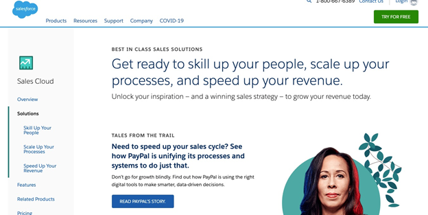
Sales Cloud is SalesForce’s top sales solution that provides several different benefits to your company by doing the following things:

Maximize revenue. Use Sales Cloud to help your company’s revenue grow by building strong and realistic monetization strategies. Sales Cloud makes available data models and workflows that are specific to your industry, so you can get the most accurate results.

Scale. Have the ability to identify shits in the market quickly and adapt your forecasts and goals quickly, easily, and with accuracy.

Accuracy. Speaking of accuracy, Sales Cloud’s forecasts will help provide you with a precise view of your entire company so you can see how things are running down the pipeline.

Performance. This solution allows you to see which sales reps are performing highest, and who may need a nudge in the right direction.

Complex forecasting. Not all forecasting is simple. In fact, most forecasting is complex. Tools available in Sales Cloud help you to keep forecasts on track and as simple as possible.

Choose the Right Method

As much as we may wish that sales forecasting was easy, the reality of it is different. What many companies struggle with is finding the forecasting method that is right for them, as all forecasts are not created equally. Each business scenario requires a different method that addresses specific needs.

Determining which forecasting method is right for your company may take some trial and error, but to make your starting place a bit easier, here are some of the most common sales forecasting methods.

Trend-based sales forecasting. This method looks at the history of your sales team’s performance and determines from that what revenue may look like in the future.

Opportunity stages forecasting. This approach to forecasting is best for assessing deals that you currently have in your pipeline. It allows you to quickly and easily estimate incoming revenue and get an objective understanding of where your team is at. Additionally, this method is beneficial for assessing your sales team’s performance and seeing where there is room for improvement.

Length of the sales cycle. This forecasting method helps a company to understand the different steps in a sales process and the timeline that accompanies those steps. This includes when a deal starts, when it’s projected to end, where the team is in the process, and what needs to be done to close. This quantitative method is best for predicting when a deal will close, based on the actual amount of time the deal has been in progress.

Regression analysis. This analysis of your sales is influential in revealing information about your company that will hopefully aid in future growth. It is a quantitative method that reviews factors that may be negatively affecting sales. With this knowledge, your team can make changes to the sales process that will help everyone to better reach goals.

Forecast stages. If you require an inside look at how your sales team feels about deals, this is the forecasting method for you. It is a quantitative approach that helps to individually assess sales reps’ techniques based on insights and information from the reps themselves, rather than from a deal that is already working its way through pre-determined stages.

Scenario writing. This forecasting approach is a qualitative one that is best used for long-term planning. It is achieved by projecting what you think is a likely outcome, based on a set of assumptions – things like worst-case and best-case scenarios. It is similar to a contingency plan that allows you to plan accordingly.

Excel/Google Sheets

Excel and Google Sheets are reliable tools in letting you create sales forecasts cheaply and easily. We prefer Google Sheets, as it automatically saves and can easily be shared with your team. Updates to Google Sheets are made immediately and there is no need to email versions of the spreadsheets back and forth.

Analytics Software

Analytics software provides the ability to create a sales forecast thanks to the features available. Something like Zoho Analytics is a simple way to utilize forecasting algorithms and past sales data to create accurate forecasts.

The Basics of Sales Forecasting

Making a sales forecast doesn’t have to be complicated, as long as you have the basics down. If you are choosing to go the manual route and create one on your own, here are the step-by-step instructions and basic information you need to know.

Determine Your Forecast Time Period

The method and way you plan to use your sales forecasting determine how far ahead your forecast projects. It could be monthly, quarterly, annually, or a longer period.

In the beginning, as you start in the world of sales forecasting, it is advised to estimate in a shorter period (monthly or quarterly) so you can focus on accuracy for that time before you extend it to annually or longer.

List Your Products/Services

Part of forecasting is writing down all the products and/or services that your company offers. If necessary, put them in categories so that you can predict sales for each category. This better sets you up for success in establishing your forecast and projecting profit.

Calculate Unit Sales Prediction

This step in the process requires a realistic prediction of how many units your team will sell in the time period you’re focusing your forecast on. One way you can do this is by using historical data and by making changes to that depending upon what you expect the demand to be in the period you’re forecasting for.

Also, look at outside factors that could affect sales. This may things such as new product or service launches, changes in the economy, the time of year (holidays, etc.), and more.

Multiply By Selling Price

Once you have the above things determined, multiply the predicted number of unit sales by the average selling price. The average selling price (ASP) is something that you can calculate by taking a look at your sales history and adjusting the price for factors such as inflation.

Repeat

To complete the forecast, repeat the above steps for each category of products and/or services and each interval of time you are forecasting for. It is important to keep in mind that the further out you go in your sales forecast, the more room for error there is. Thus, as time goes on and the time intervals you predicted get closer to occurring, you want to add in the real values and adjust your forecasts.

This means that, if you find you low-balled your sales forecast for the first quarter of the year, then you want to increase your forecasted sales by that amount for the remainder of the time intervals.

5 Tricks for Sales Forecasting

The goal of sales forecasting is not to just get a forecast set up for the sake of having one, but to establish an accurate forecast that will give your company a strong idea of what to expect in terms of sales for a determined period in the future.

To get the most precise sales forecast possible, here are some tricks to guide you.

Establish a Process

If you want your team to accurately predict the chances of closing, then you need a sales process that is consistent and has the same stages and steps. Everyone needs to be on the same page and work as a team to reach success. This requires your team to agree on counting leads and when to enter and exit the sales funnel.

Set Quotas

Sales quotas serve as a strong base with which you can compare your sales forecasting. Quotas are also important to help your team understand goals and to help your company keep track of performance. To get the most success out of quotas, they need to be set for both individuals and teams.

Invest in CRM Software

As mentioned above, customer relationship management software (CRM) such as Salesforce or Zoho provides your sales team with a database where they can track opportunities. This allows you to create more accurate predictions of sales, which is great for your team and your company as a whole in the short and long term.

Choose a Method

Once you have the above steps in place, then you want to choose a sales forecasting method that works best for your team’s specific needs. Before picking the method that is right for you, take a look at your team, your business plan, historical data, current data, industry standards, and more. All these variables will help you build a strong and accurate sales forecasting model.

Keep Your Sales Team Informed

One of (if not the) most important part of a successful sales forecast is maintaining communication with your team and keeping them in the loop. This means letting them know of any changes or decisions as soon as they happen. One of the easiest ways to do this is by using CRM software. This solution keeps your team informed of what’s going on without having to deal with flooding inboxes with email updates.

On the other side of the coin, make sure that your team provides you with their input on what is working with the process and what could use some adjusting. Maintaining communication between all members of the team and all levels is essential to the success of your sales forecast, your sales, and your revenue.

How to Use Notion with Gmail and Google Sheets using Apps Script

Notion, my absolute favorite tool for storing all sorts of things from web pages to code snippets to recipes, just got better. They’ve released a public API and thus it will be a lot easier for developers to read and write to their Notion workspace from external apps.

For instance, you can create a document in Google Docs and export it to Notion while staying inside Docs. Google Sheets users can pull pages from Notion database into their spreadsheet. Any new submissions in Google Forms can be directly saved to Notion and so on!

Save Gmail Messages in Notion

I have put together a Gmail add-on that makes it easy for you to save email messages, or any other text content, from Gmail to your Notion workspace with a click. Here’s how the app works.

Step 1: Connect Gmail to Notion

002815

Step 2: Allow Access to Notion pages - if you have multiple databases in your Notion workspace, you have an option to grant access to select databases and the rest will be inaccessible to the external app.

Authorize Notion

Step 3: Choose Email - open any email message in Gmail and you’ll have an option to edit the content of the email subject and body before sending the content to your Notion page. Please note that the app only supports plain text format at this time.

Send Email to Notion

Step 4: Open Notion - As soon as you hit the Send to Notion button, the content of the currently selected email message is added to your Notion database. You can click the All updates link in your Notion sidebar to view to recently added page.

Notion page

If you would like to try this Gmail to Notion app, please get in touch.

How to Use Notion with Google Apps Script

If you would to integrate your own Google add-on with Notion API, here’s a brief outline of the steps involved.

  1. Go to notion.so and click the Create New Integration button. You’ll be provided with a Client ID and Client Secret that you’ll need in a later step.

  2. Include the OAuth2 library in your Apps Script project and invoke the getRedirectUri method to get the OAuth2 redirect URL for the previous step.

const getNotionService = () => {
  return OAuth2.createService("Notion")
    .setAuthorizationBaseUrl("https://api.notion.com/v1/oauth/authorize")
    .setTokenUrl("https://api.notion.com/v1/oauth/token")
    .setClientId(CLIENT_ID)
    .setClientSecret(CLIENT_SECRET)
    .setCallbackFunction("authCallback")
    .setPropertyStore(PropertiesService.getUserProperties())
    .setCache(CacheService.getUserCache())
    .setTokenHeaders({
      Authorization: `Basic ${Utilities.base64Encode(
        `${CLIENT_ID}:${CLIENT_SECRET}`
      )}`,
    });
};

const authCallback = (request) => {
  const isAuthorized = getNotionService().handleCallback(request);
  return HtmlService.createHtmlOutput(
    isAuthorized ? "Success!" : "Access Denied!"
  );
};

const getRedirectUri = () => {
  console.log(OAuth2.getRedirectUri());
};
  1. Connect to Notion API - Make a Get HTTP request to the /vi/databases to fetch a list of all databases that the user has explicitly shared with authorized app.
function getDatabasesList() {
  var service = getNotionService();
  if (service.hasAccess()) {
    const url = "https://api.notion.com/v1/databases";
    const response = UrlFetchApp.fetch(url, {
      headers: {
        Authorization: `Bearer ${service.getAccessToken()}`,
        "Notion-Version": "2021-05-13",
      },
    });
    const { results = [] } = JSON.parse(response.getContentText());
    const databases = results
      .filter(({ object }) => object === "database")
      .map(({ id, title: [{ plain_text: title }] }) => ({ id, title }));
    console.log({ databases });
  } else {
    console.log("Please authorize access to Notion");
    console.log(service.getAuthorizationUrl());
  }
}

Gmail to Notion - Try the App

The Gmail to Notion app is in private beta. If you would like to use it with your Gmail or Google Workspace account, please get in touch for an invite.

How to Perform IP Address Lookup with Google Sheets

Websites can determine the visitor’s geographic location using their IP address and serve more relevant content. For example, a weather website may use your IP address to estimate your approximate location and provide weather forecast for your current city automatically. A currency exchange website can determine your default currency based on your country which is detected from your IP address.

Google Sheets - IP 2 Location

There are free web IP lookup services, ip2c.org for example, that will reveal the country of your client’s IP address with a simple HTTP request. We internally use that service at Digital Inspiration to determine the payment service provider on the checkout page.

Bulk IP Lookup with Google Sheets

IP2Location is another good alternative that retrieves more detailed geolocation information for any IP address. The IP location lookup service can retrieve the client’s country, city name, region, the ISP name and more.

If you have a bulk list of IP addresses, you can use Google Sheets to estimate the corresponding geographic details for each of the addresses in few easy steps:

  1. Click here to make a copy of the Google Sheet for performing IP lookups in bulk.

  2. Paste the list of IP addresses in column A, one per row. The lookup service works for both IPv4 and IPv6 addresses.

  3. Enter your key in cell E1. If you have a small list of IP address, use demo as the key or get your own API key from ip2location.com.

  4. Click the Run button, authorize the script and watch as the geographic details and ISP names are populated in the sheet.

IP2Location Web Service Demo

How IP2Location Script Works

Internally, the Google Sheet uses the IP2location web service with Google Apps Script to transform IP addresses into geographic region.

It uses the UrlFetchApp service to perform multiple HTTP requests in a single batch for improved performance. Here’s the full source code:

const ip2location = () => {
  // Get all the input data from Google Sheet
  const ss = SpreadsheetApp.getActiveSheet();
  const data = ss.getDataRange().getDisplayValues();

  // Use your own API key or use demo key
  const apiKey = data[0][4] || "demo";

  // Generate API URL for IP address
  const getUri_ = (ipAddress) => {
    const API_URL = "https://api.ip2location.com/v2";
    return `${API_URL}/?ip=${ipAddress}&key=${apiKey}&package=ws4`;
  };

  const requests = [];

  for (let r = 2; r < data.length; r++) {
    const [ipAddress, countryName] = data[r];
    // Only process rows where the country is blank
    if (ipAddress && !countryName) {
      requests.push({ url: getUri_(ipAddress), rowNumber: r + 1 });
    }
  }

  // Make API calls in bulk using the UrlFetchApp service
  UrlFetchApp.fetchAll(requests).forEach((content, i) => {
    // Parse the JSON response
    const { city_name, country_name, isp, response } = JSON.parse(content);

    // If the response is populated, the API call failed
    if (response) throw new Error(response);

    // Write the response data to Google Sheet
    const values = [[country_name, region_name, city_name, isp]];
    ss.getRange(requests[i].rowNumber, 2, 1, 4).setValues(values);
  });

  // Flush all changes
  SpreadsheetApp.flush();
};

How to Copy a Formula Down an Entire Column in Google Sheets

You are working inside a Google Spreadsheet where a formula needs to copied down to the last row of the sheet. You also need the formula to be added automatically when a new row is added to the Google Sheet.

There are several ways to solve this problem.

Copy Formula Down in Google Sheets

The easiest approach to copy down formulas is to use the fill handle in Google Sheets. Write your formula in the first row of your spreadsheet, and then point your mouse to the lower right corner of the formula cell.

fill-down-sheet-formula.gif

The pointer changes into a fill handle (black plus symbol) that you can drag to the last row of the sheet. The fill handle will not just copy down the formulas to all the adjacent cells but also copies the visual formatting.

If you need to copy the formulas across cells but sans any formatting, select the cell that contains the formatting and press Ctrl+C to copy it to the clipboard. Next, select the range where that formula needs to applied, right-click, choose Paste Special and Paste Formula only.

copy-formula-without-formatting.png

Apply Formula to the Entire Column in Google Sheets

If you have hundreds of rows in a Google Spreadsheet and you want to apply the same formula to all rows of a particular column, there’s a more efficient solution than copy-paste - Array Formulas.

Highlight the first cell in the column and type the formula as earlier. However, instead of specifying a single cell as a parameter, we’ll specify the entire column using the B2:B notation (start from cell B2 and go all the way down to the last row of column B).

Then press Ctrl+Shift+Enter, or Cmd+Shift+Enter on Mac, and Google Sheets will automatically surround your formula with ARRAYFORMULA function.

arrayformula.gif

Thus, we could apply the formula to the entire column of the spreadsheet with only a single cell. Array Formulas are more efficient as they process a batch of rows in one go. They are also easier to maintain as you only need to modify a single cell to edit the formula.

One issue that you may have noticed with the above formulae is that it applies to every row in the column where you have only want to add formulas to rows that contain data and skip the blank rows.

This can be done by adding an IF contain to our ARRAYFORMULA so that it doesn’t apply the formula the any of the blank rows.

Google Spreadsheet offers two functions to help test whether a cell is empty or now.

  • ISBLANK(A1) - Returns TRUE if the referenced cell is empty.
  • LEN(A1) <> 0 - Returns TRUE if the referenced cell not empty, FALSE otherwise

Our modified Array Formulas would therefore read:

Using ISBLANK(Cell Reference):

arrayformula-isblank.png

There are several other ways to test if a cell is blank or not:

=ArrayFormula(IF(ISBLANK(B2:B), "", ROUND(B2:B*18%, 2)))
=ArrayFormula(IF(LEN(B2:B)<>0, ROUND(B2:B*18%, 2), ""))
=ArrayFormula(IF(B2:B="", "", ROUND(B2:B*18%, 2)))

Use Array Formulas inside Column Headers

In our previous examples, the text of the column titles (like Tax, Total Amount) was pre-populated and the formulas were only added to the first row of the dataset.

We can further improve our formula so that they can be applied to the column header itself. If the index of the current row is 1, calculated using the ROW() function, the formula outputs the column title else it performs the calculation using the formula.

=ArrayFormula(IF(ROW(B:B)=1,"Tax",IF(ISBLANK(B:B),"",ROUND(B:B*18%, 2))))

arrayformula-first-row.png

Auto Fill Formulas into Google Form Submissions

ARRAYFORMULA functions are particularly useful for Google Forms when the form responses are getting saved inside a Google Sheet. You cannot do live calculations inside Google Forms but they can be performed inside the spreadsheet that is collecting the responses.

You can create new columns inside the Google Spreadsheet and apply the ARRAYFORMULA to the first row of the added columns.

When a new form submission is received, a new row would be added to the Google Sheet and the formulas would be cloned and automatically applied to the new rows without you have to copy-paste stuff.

Also see: Convert Google Form Response to PDF Documents

How to Use VLOOKUP inside ARRAYFORMULA

You can combine ARRAYFORMULA with VLOOKUP to quickly perform a lookup across an entire column.

Say you have a “Fruits” sheet that lists the fruit names in column A and the corresponding prices in column B. The second sheet “Orders” has fruit names in column A, the quantity in column B and you are supposed to calculate the order amount in column C.

arrayformula-vlookup.png

=ArrayFormula(
  IF(ROW(A:A)=1,
  "Total",
  IF(NOT(ISBLANK(A:A)), VLOOKUP(A:A, Fruits!A2:B6, 2, FALSE) * B:B, "")))

In simple English, if the row of the current cell is 1, output the column title in plain text. If the row is greater than 1 and the column A of the current row is not empty, perform a VLOOKUP to fetch the price of the item from the Fruits sheet. Then multiply that price with the quantity in cell B and output the value in cell C.

If your VLOOKUP range is in another Google Spreadsheet, use the IMPORTRANGE() function with the ID of the other Google Sheet.

Please note that you may have to use semicolons in the spreadsheet formulas instead of commas for some locales.

The Principles Of Visual Communication

Visual storytelling can be intimidating. We’re taught to communicate with words, but words are not always the best way to convey information and ideas. Sometimes the best way to tell stories is through thoughtfully crafted visuals, not long paragraphs of text. Creating visuals is not reserved for designers, illustrators, or artists. It’s a skill anyone can learn and put into practice every day.

The key to becoming more comfortable with visual communication is unlearning the rules you’ve subconsciously collected. Growing up, I loved creating rainbow text with WordArt, adding fancy document borders, and downloading decorative fonts on Dafont. My work in grade school all looked like this:

I was just playing with fonts and styles for fun. I had no notion of what makes up "good" or "bad" visual design. Looking back at this poem, the typography is objectively difficult to read. However, I intentionally found fonts that matched each adjective and made each heading the same font style. Through these moments of play, I started to build the foundation of my visual intuition.

Visual storytelling is the process of conveying ideas using things you can see. As we get older, visual storytelling becomes more intimidating because we’re conditioned to believe visuals are childish or purely decorative. We’re taught that all writing needs to be in 12pt Times New Roman and double spaced on letter-sized paper. We’re told that it’s “more professional” to minimize exclamation marks and emojis. We make excuses like “I’m just not artistic enough.”

Today, I communicate with visuals daily. I guide emerging designers to develop their visual intuitions and I design products for homeschooling families. Becoming a better visual storyteller is all about balancing play and practice with a foundation of principles. It’s about finding the happy medium between having fun with WordArt and playing it safe with Times New Roman.

In this article, we will explore visual principles, highlight why visual storytelling is a valuable skill for everyone to learn, and demonstrate how you can improve your visual storytelling through play.

Show > Tell

All visual storytelling can be broken down into a set of concrete principles. To ease you into the topic, let’s learn how typography sets the foundation for all visual storytelling and examine principles shared in effective visuals.

Typography Sets The Foundation

You don’t always need to add an illustration or graphic to visually communicate an idea! Good typography sets the foundation for all visual storytelling. There are plenty of typography resources out in the wild, but my two biggest pieces of advice are:

  1. Stick to one typeface.
    Find a typeface with multiple weights and styles. Combining different typefaces is difficult. My favorite Google fonts right now are IBM Plex Sans and Inter.
  2. Change one thing at a time.
    Creating enough contrast between type styles is an art. My recommendation is to change just one axis at a time: size, weight, style, and color are the most popular things to change.

Here’s an example of visual storytelling using simply typography.

  • In version 1, I use the same style for the entire body of the text.
  • In version 2, I bold the most important text on the page: "Change one thing at a time"
  • In version 3, I decrease the paragraph text size and move the heading to its own line.
  • In version 4, I highlight the word "one" in pink to signify importance and I make the paragraph text a lighter shade of gray.

Small tweaks to typography can often communicate more than adding more words. Before you consider adding a visual, always experiment with the typography first. Typography is more than selecting a font. You can change the importance of text by adjusting the size, weight, composition, and color. Think about what is most important and make sure that stands out in a body of text.

Resources On Typography

What Do Good Visuals Have In Common?

Good visuals have focus, communicating the most important idea at a glance. Reports should be informative, but easy to scan. Flowcharts should highlight differences between old and new processes. When you’re creating a visual, it can be easy to overwhelm the audience with too many ideas at once. The best visuals maintain a clear message by drawing attention to what’s most important.

I’ve spent a lot of time mentoring emerging product designers on portfolio building. Design portfolios typically consist of a few case studies that walk through a designer’s thought process from beginning to end.

Below are two low fidelity sketches of portfolio case studies. This is an exaggeration, but the one on the left is less successful because there are no visuals to accompany the story. The one on the right is easier to scan because there are images showing the designer’s process.

Good visual communicators can highlight the most important parts of a visual. In the case studies graphic above, I intentionally blocked out the body text and made the two versions nearly identical. I tried to minimize all visual distractions. If I add filler body text, the graphic is harder to comprehend because it becomes visually cluttered.

Visuals can also be helpful when you need to communicate a change in the process. For example, if your company restructures the hiring process, it might be helpful to show a before-and-after flowchart that highlights the changes. Imagine these are the changes:

  • We moved the technical interview from the second to the first step;
  • We added a behavioral interview as the last step;
  • We now require at least one strong hire for a candidate to get an offer.

This might seem obvious, but we tend to default to emails and documents in the workplace. Before and after visuals are great because they help people visualize the differences.

In the example below, you’ll notice that I use color sparingly as a way to highlight new additions to the process. Color is one of the best ways to draw attention to important aspects of a visual.

You can create a graphic with anything including pen and paper! I used Figma for the one above because I’m familiar with the tool, but you can create a similarly effective visual with something as simple as Google Sheets.

Visuals are a tool you can use to add clarity to any idea. Remember that you don’t always have to add a graphic or illustration. You can communicate a lot with just small tweaks to typography and presentation. Just make sure to focus on the most important idea and make sure it shines through.

Tools For Creating Visuals
  • Figma has a higher learning curve but offers the most flexibility.
  • Whimsical is easy to use and has templates for creating common visuals like flowcharts.
  • Mural is like a digital whiteboard. It’s great for collaboration and has templates.

Developing Visuals Through Play

Developing visuals takes time, play, and experimentation. If you’re creating visuals from scratch, your first attempt will never be the best one! I’ve been in the design industry for a while now and I still fail and iterate every single day. This is a screenshot of my recent design iterations for just one screen in a flow.

Learning how to become a better visual storyteller is all about practice and iteration. In my design classes, I teach students to iterate by making it into a competition. I separate the students into teams and the goal is for each team to get the most iterations in a set period of time. For this activity, I encourage students to change one thing at a time as they iterate.

This exercise teaches students to be comfortable trying lots of things that might not work. After 15 minutes of iterating, I have the groups discuss which designs are their favorites. Why do you feel the designs you chose are the most effective?

Iterating might seem daunting, but it’s actually a really fun process. When you’re developing a visual, start by thinking about the one thing you want the audience to learn. Imagine that our goal is to communicate that you need to stay 6-feet apart to prevent the spread of Covid-19.

I always start with setting typography first. Here is a series of iterations where I only adjust the font size, weight, and style.

For each iteration, I only changed one thing! Which version do you think works the best? Personally, I think the last iteration works best because the message is loud and clear. Next, I experimented with a few different typefaces. Every typeface has a different personality:

After experimenting with type, we can experiment with adding a graphic or illustration to the poster. You don’t have to be an illustrator to create a graphic. There are plenty of resources online that you can use to compose a graphic.

  • In version 1, I used Apple emojis.
  • In version 2, I drew an icon of a person using two circles and a rectangle.
  • In version 3, I used an illustration library Humaaans.
  • In version 4, I used Apple’s symbols set.

These directions are all effective. Directions 2 and 4 feel more like an official government graphic, but directions 1 and 2 feel more fun and inviting. With all our components in place, we can try adding style and color. It’s important to use style and color sparingly because they can overwhelm the message.

All four of these iterations work well! Directions (2) and (4) capture the eye of the viewer because they use a solid block of color in the background. Directions (1) and (3) might be easier to scan because of the simplicity of the background. I like how direction (3) uses purple to highlight the "6 feet" guidelines.

This is what San Francisco’s "Stay 6 feet apart" poster actually looks like. It communicates the message pretty well. The most important text "Stay 6 feet apart" is highlighted in yellow and it also includes a simple graphic that reemphasizes the message.

Resources For Developing Visuals

What’s Next?

The next time you design a slide deck, make a poster or create a document, think about incorporating a piece of visual storytelling. Start small by emphasizing important parts of the text with typography. If you decide to add a visual, remember that you don’t have to use fancy tools. Try starting with a pencil and paper or any tool you’re familiar with. Visual storytelling is all about communicating ideas, not creating works of art.

If you’re unsure where to start below are some fantastic resources:

Anyone can learn to communicate with visuals! I recommend sharing your work with friends or peers to see if your message is getting across. Getting feedback early and often will improve your work and ideas. The more you iterate, the faster and better you’ll get in the future. With practice and play, you’ll start to collect your own visual principles and build your own visual foundation.

How to Preserve Formatting of Spreadsheet Cells in Mail Merge

The Mail Merge app merges data from a Google Spreadsheet and sends them as personalized emails. You can format your sheet data in multiple colors, choose different font families, vary the size of your text, include hyperlinks, line breaks and more.

The rich text of spreadsheet cells is internally translated into HTML tags with inline CSS and thus the cell formatting is preserved in the outgoing Gmail messages. Here’s an example:

Rich Text Email in Gmail

If you would like to enable this feature, go to the Add-ons menu in Google Sheets > Mail Merge with Attachments > Configure Mail Merge and check the “Preserve Cell Formatting” option.

You can even format your spreadsheet cells with conditional formatting and the text styles will be retained in mail merge. For instance, you can dynamically color the invoice amount column in red and make it bold if the due date has passed and this value would show up in bold red in the email message as well.

Send Rich Text HTML Emails with Google Sheet

This snippet handles the transformation of rich-text Spreadsheet data to HTML. The functions reads the data from a cell, specified in A1 notation, breaks the rich text into blocks that have the same text styles and translate individual blocks into HTML tags.

const sendRichEmail = () => {
  const cellAddress = 'A1';
  const sheetName = 'Mail Merge';
  const recipient = 'amit@labnol.org';

  const richTextValue = SpreadsheetApp.getActiveSpreadsheet()
    .getSheetByName(sheetName)
    .getRange(cellAddress)
    .getRichTextValue();

  /* Run is a stylized text string used to represent cell text.
     This function transforms the run into HTML with CSS
   */
  const getRunAsHtml = (richTextRun) => {
    const richText = richTextRun.getText();

    // Returns the rendered style of text in a cell.
    const style = richTextRun.getTextStyle();

    // Returns the link URL, or null if there is no link
    // or if there are multiple different links.
    const url = richTextRun.getLinkUrl();

    const styles = {
      color: style.getForegroundColor(),
      'font-family': style.getFontFamily(),
      'font-size': `${style.getFontSize()}pt`,
      'font-weight': style.isBold() ? 'bold' : '',
      'font-style': style.isItalic() ? 'italic' : '',
      'text-decoration': style.isUnderline() ? 'underline' : '',
    };

    // Gets whether or not the cell has strike-through.
    if (style.isStrikethrough()) {
      styles['text-decoration'] = `${styles['text-decoration']} line-through`;
    }

    const css = Object.keys(styles)
      .filter((attr) => styles[attr])
      .map((attr) => [attr, styles[attr]].join(':'))
      .join(';');

    const styledText = `<span style='${css}'>${richText}</span>`;
    return url ? `<a href='${url}'>${styledText}</a>` : styledText;
  };

  /* Returns the Rich Text string split into an array of runs,
  wherein each run is the longest possible
  substring having a consistent text style. */
  const runs = richTextValue.getRuns();

  const htmlBody = runs.map((run) => getRunAsHtml(run)).join('');

  MailApp.sendEmail(recipient, 'Rich HTML Email', '', { htmlBody });
};

Known Limitations

You can format the cells of your Google Spreadsheet in any font family - from the cursive Caveat to the heavy Impact typeface - but if the recipient doesn’t have these fonts installed on their computer, the rendered text in the email would fallback to the default font.

The font colors, font size and text styles (bold, italics, underline) get perfectly transformed into HTML but other properties like background fill colors, borders and text-alignment of the cell are ignored.

Also, if your spreadsheet cells are formatted as dates, the rich text functions may not work.

How to Highlight Duplicates in Google Sheets and Remove

The Email Extractor app pulls emails addresses of your contacts from Gmail into a Google Sheet. You can then use Mail Merge or Document Studio to send personalized emails to your contacts from within the sheet itself.

That said, the imported mailing list may sometimes have duplicate email addresses and it is thus be a good idea to clean up the data in your Google Sheet by removing duplicates before sending out the emails.

Highlight Duplicates in Google Sheets

You can use Conditional Formatting in Google Sheets combined with the COUNTIF formula to quickly highlight cells that contain duplicate values.

Highlight Duplicates in Google Sheets

Here’s how you can find duplicates in Google Sheets:

  1. Open the Google Sheet containing your data and go to the Format menu.

  2. Select Conditional Formatting from the expanded menu. This will help us change the colors of cells, rows or columns that meet a specific criteria.

  3. In the Apply to Range input box, add the range of cells that contain possible duplicates. In our case, the email addresses are in column A so we can put A:A to specify the entire A column.

  4. Under the ‘Format cells if’ section, choose “Custom formula is” from the dropdown list as set the formula as =COUNTIF(A:A, A1) > 1

Click the Done button and you’ll instantly notice that all duplicate cells are highlighted as shows in the screenshot below.

Duplicate Cells in Google Spreadsheet

The COUNTIF Function

The COUNTIF function in Google sheets (and Microsoft Excel) essentially counts the number of cells in the range that meet a specific criteria. For instance =COUNTIF(A:A, "apple") will count the number of cells that contain the word apple.

It can accept wildcard characters too so =COUNTIF(A:A, "apple?") will count cells that contain the word apple or apples. Or say =COUNTIF(A:A, "*@gmail.com") and it will highlight all email address that end with a gmail address.

Please note that the COUNTIF function is case-insensitive so values like gmail.com and Gmail.com are seen as duplicates.

Highlight Entire Row Containing Duplicates

If you’ve noticed in the previous screenshot, only specific cells that have duplicate values are highlighted through conditional formatting.

However, if you would like the Google Sheet to highlight the entire spreadsheet row that contains duplicate values, we need to slightly tweak the formatting rule.

  1. Go to the Apply to Range input box and specify the entire spreadsheet range, not just the column that contains duplicates.

  2. In the custom formula,use absolute reference for the range and also change criterion to use $A1 instead of A1. When we use $A1, we are telling Google Sheet to only change the row but lock the column.

The new duplicate detection formula reads =COUNTIF($A$1:$C$50, $A1)>1

Highlight Duplicate Rows in Spreadsheet

Compare Multiple Columns for Duplicates

If you would like to determine duplicates by comparing data in multiple columns of the Google Sheet, use COUNTIFS instead of COUNTIF.

For instance, if column A is Email Address and column B is Company Name and you would like highlight duplicates cell only when the combination of values in Column A and B is identical, the new formula can be written as =COUNTIFS(A:A, A1, B:B, B1)>1

Remove Duplicate Rows in Google Sheets

Now that we have figured out a simple method to highlight duplicates in Google Sheets, the next task is to remove all duplicate rows.

There are two ways to go about it - either use Google Apps script or use the built-in feature of Google Sheets to remove duplicates.

First, highlight the entire column in Google Sheet that contains the duplicate data. Next, go to the Data menu and choose the Remove Duplicates option.

Select which columns to include and whether or not the selected range has any header row. Click Remove duplicates and your list is clean up in one go. Like with COUNTIF function, Google Sheets will ignore case and formatting when determining duplicates.

Remove Duplicate Rows

Remove Duplicates with Google Scripts

If you prefer automation, here’s a little snippet that will remove the duplicates in your active Google Sheet based on data in the first column.

/** @OnlyCurrentDoc */

function removeDuplicateRows() {
  SpreadsheetApp.getActiveSpreadsheet()
    .getActiveSheet()
    .getDataRange()
    .removeDuplicates([1]);
}

Measure Core Web Vitals of your Websites with Google Sheets

Google’s web.dev virtual conference happened last month and if there’s one key takeaway from the event, it is the “core web vitals” initiative. Website owners can no longer afford to ignore core vitals as these are now a ranking signal in Google Search.

Google Core Web Vitals

Google has long been stressing on the need to build faster web pages but with core vitals, they provide a set of actionable metrics - Largest Contentful Paint (LCP), First Input Delay (FID), and Cumulative Layout Shift (CLS) - that should be measured by website owners across mobile and desktop computers.

The session on speed tooling by Elizabeth Sweeny of the Chrome team offers a good overview of what Core Web Vitals are and she also discusses the various tools that are available for webmasters and developers to measure web vitals for their pages.

Measure Core Vitals with Google Sheets

While there are quite a few tools available to help you measure core web vitals for a website - from Chrome extensions to web apps - they have to be triggered manually and can only measure core vitals for a single website / webpage at a time.

Core Web Vitals in Google Sheets

If you are looking to automatically measure core web vitals for multiple websites, maybe that of your competitor’s websites as well, here’s a Google Sheet that can help. The spreadsheet will not only help you measure vitals for multiple URLs but you can also visualize the change in various metrics over time with the help of sparklines.

Here’s how you can get started:

  1. Click here to make a copy of the Web Vitals sheet in your Google Drive.

  2. Switch to the first tab and enter a list of URLs that you would like to measure and track. Also provide unique sheet names for each URL and the metrics for that URL will get stored in the corresponding sheet.

  3. Click the “Track Core Vitals” button, authorize the sheet and you’re all set.

The button will set up a daily cron job that will automatically connect to Google’s PageSpeed API, fetch the core vitals for each specified URL and write them to the corresponding sheet.

The Apps Script source code is available on Github. As always, you are free to reuse, modify and publish the code based on your own requirements.

Core Web Vitals App

Google Maps Formulas for Google Sheets

You can bring the power of Google Maps to your Google Sheets using simple formulas with no coding. You don’t need to sign-up for the Google Maps API and all results from Google Maps are cached in the sheet so you are unlikely to hit any quota limits.

To give you a quick example, if you have the starting address in column A and the destination address in column B, a formula like =GOOGLEMAPS_DISTANCE(A1, B1, "driving") will quickly calculate the distance between the two points.

Or modify the formula slightly =GOOGLEMAPS_TIME(A1, B1, "walking") to know how long it will take for a person to walk from one point to another.

If you would like to try the Google Maps formulas without getting into the technical details, just make a copy of this Google Sheet and you are all set.

Google Maps in Google Sheets

Using Google Maps inside Google Sheets

This tutorial explains how you can easily write custom Google Maps functions inside Google Sheets that will help you:

  1. Calculate distances between two cities or any addresses.
  2. Calculate the travel time (walking, driving or biking) between two points.
  3. Get the latitude and longitude co-ordinates of any address on Google Maps.
  4. Use reverse geocoding to find the postal address from GPS co-ordinates.
  5. Print driving directions between any points on earth.
  6. Get the address from the zip code itself.

1. Calculate Distances in Google Sheets

Specify the origin, the destination, the travel mode (walking or driving) and the function will return the distance between the two points in miles.

=GOOGLEMAPS_DISTANCE("NY 10005", "Hoboken NJ", "walking")

/**
 * Calculate the distance between two
 * locations on Google Maps.
 *
 * =GOOGLEMAPS_DISTANCE("NY 10005", "Hoboken NJ", "walking")
 *
 * @param {String} origin The address of starting point
 * @param {String} destination The address of destination
 * @param {String} mode The mode of travel (driving, walking, bicycling or transit)
 * @return {String} The distance in miles
 * @customFunction
 */
const GOOGLEMAPS_DISTANCE = (origin, destination, mode) => {
  const { routes: [data] = [] } = Maps.newDirectionFinder()
    .setOrigin(origin)
    .setDestination(destination)
    .setMode(mode)
    .getDirections();

  if (!data) {
    throw new Error('No route found!');
  }

  const { legs: [{ distance: { text: distance } } = {}] = [] } = data;
  return distance;
};

2. Reverse Geocoding in Google Sheets

Specify the latitude and longitude and get the full address of the point through reverse geocoding of coordinates.

=GOOGLEMAPS_DISTANCE("NY 10005", "Hoboken NJ", "walking")

/**
 * Use Reverse Geocoding to get the address of
 * a point location (latitude, longitude) on Google Maps.
 *
 * =GOOGLEMAPS_REVERSEGEOCODE(latitude, longitude)
 *
 * @param {String} latitude The latitude to lookup.
 * @param {String} longitude The longitude to lookup.
 * @return {String} The postal address of the point.
 * @customFunction
 */

const GOOGLEMAPS_REVERSEGEOCODE = (latitude, longitude) => {
  const { results: [data = {}] = [] } = Maps.newGeocoder().reverseGeocode(latitude, longitude);
  return data.formatted_address;
};

3. Get the GPS coordinates of an address

Get the latitude and longitude of any address on Google Maps.

=GOOGLEMAPS_LATLONG("10 Hanover Square, NY")

/**
 * Get the latitude and longitude of any
 * address on Google Maps.
 *
 * =GOOGLEMAPS_LATLONG("10 Hanover Square, NY")
 *
 * @param {String} address The address to lookup.
 * @return {String} The latitude and longitude of the address.
 * @customFunction
 */
const GOOGLEMAPS_LATLONG = (address) => {
  const { results: [data = null] = [] } = Maps.newGeocoder().geocode(address);
  if (data === null) {
    throw new Error('Address not found!');
  }
  const { geometry: { location: { lat, lng } } = {} } = data;
  return `${lat}, ${lng}`;
};

4. Print the driving directions between addresses

Specify the origin address, the destination address, the travel mode and the function will use the Google Maps API to print step-by-step driving directions.

=GOOGLEMAPS_DIRECTIONS("NY 10005", "Hoboken NJ", "walking")

/**
 * Find the driving direction between two
 * locations on Google Maps.
 *
 * =GOOGLEMAPS_DIRECTIONS("NY 10005", "Hoboken NJ", "walking")
 *
 * @param {String} origin The address of starting point
 * @param {String} destination The address of destination
 * @param {String} mode The mode of travel (driving, walking, bicycling or transit)
 * @return {String} The driving direction
 * @customFunction
 */
const GOOGLEMAPS_DIRECTIONS = (origin, destination, mode = 'driving') => {
  const { routes = [] } = Maps.newDirectionFinder()
    .setOrigin(origin)
    .setDestination(destination)
    .setMode(mode)
    .getDirections();
  if (!routes.length) {
    throw new Error('No route found!');
  }
  return routes
    .map(({ legs }) => {
      return legs.map(({ steps }) => {
        return steps.map((step) => {
          return step.html_instructions.replace(/<[^>]+>/g, '');
        });
      });
    })
    .join(', ');
};

5. Measure the trip time with Google Maps

Specify the origin address, the destination address, the travel mode and the function will measure your approximate trip time between the specified addresses, provided a route exists.

=GOOGLEMAPS_DURATION("NY 10005", "Hoboken NJ", "walking")

/**
 * Calculate the travel time between two locations
 * on Google Maps.
 *
 * =GOOGLEMAPS_DURATION("NY 10005", "Hoboken NJ", "walking")
 *
 * @param {String} origin The address of starting point
 * @param {String} destination The address of destination
 * @param {String} mode The mode of travel (driving, walking, bicycling or transit)
 * @return {String} The time in minutes
 * @customFunction
 */
const GOOGLEMAPS_DURATION = (origin, destination, mode = 'driving') => {
  const { routes: [data] = [] } = Maps.newDirectionFinder()
    .setOrigin(origin)
    .setDestination(destination)
    .setMode(mode)
    .getDirections();
  if (!data) {
    throw new Error('No route found!');
  }
  const { legs: [{ duration: { text: time } } = {}] = [] } = data;
  return time;
};

Google Maps Functions in Sheets

Tip: Improve Formula Performance by Caching

The Google Sheets functions internally use the Google Maps API to calculate routes, distances and travel time. Google offers a limited quota for Maps operations and if your sheet performs too many queries in a short duration, you are likely to see errors like ""Service invoked too many times for one day” or something similar.

To get around the quota issue, it is recommended that you use Apps Script’s built-in cache to store results and, if the results of a function already exist in the case, you’ll make one less request to Google Maps.

The Maps functions inside this Google Sheet also use caching and here’s how you can implement it.

// The cache key for "New York" and "new york  " should be same
const md5 = (key = '') => {
  const code = key.toLowerCase().replace(/\s/g, '');
  return Utilities.computeDigest(Utilities.DigestAlgorithm.MD5, key)
    .map((char) => (char + 256).toString(16).slice(-2))
    .join('');
};

const getCache = (key) => {
  return CacheService.getDocumentCache().get(md5(key));
};

// Store the results for 6 hours
const setCache = (key, value) => {
  const expirationInSeconds = 6 * 60 * 60;
  CacheService.getDocumentCache().put(md5(key), value, expirationInSeconds);
};

/**
 * Calculate the travel time between two locations
 * on Google Maps.
 *
 * =GOOGLEMAPS_DURATION("NY 10005", "Hoboken NJ", "walking")
 *
 * @param {String} origin The address of starting point
 * @param {String} destination The address of destination
 * @param {String} mode The mode of travel (driving, walking, bicycling or transit)
 * @return {String} The time in minutes
 * @customFunction
 */
const GOOGLEMAPS_DURATION = (origin, destination, mode = 'driving') => {
  const key = ['duration', origin, destination, mode].join(',');
  // Is result in the internal cache?
  const value = getCache(key);
  // If yes, serve the cached result
  if (value !== null) return value;
  const { routes: [data] = [] } = Maps.newDirectionFinder()
    .setOrigin(origin)
    .setDestination(destination)
    .setMode(mode)
    .getDirections();
  if (!data) {
    throw new Error('No route found!');
  }
  const { legs: [{ duration: { text: time } } = {}] = [] } = data;
  // Store the result in internal cache for future
  setCache(key, time);
  return time;
};

Also see: Embed Google Maps in Emails and Documents

How to Enable Third-party Cookies in Google Chrome

The newer versions of Google Chrome block third-party cookies by default. Cookies are considered “bad” as they are mostly used for tracking users on the Internet but some cookies serve a useful purpose as well.

For instance, a GSuite add-on may open a small sidebar inside Google Sheets and this sidebar may need to communicate with other windows that are opened by the same add-on. Since the windows are on different domains, the only way for them to communicate with each other is through third-party cookies.

This video explains why some third-party cookies are necessary and how you can selectively allow cookies inside Google Chrome.

GSuite add-ons including Document Studio, Form Notifications and Mail Merge require you to enable third-party cookies in your browser to save user preferences and settings.

Allow Third-party Cookies for GSuite

Here are step-by-step instructions on how to enable third-party cookies in your Google Chrome browser. This will only allow cookies for GSuite add-ons in Google Sheets, Form, Docs, and Google Sides.

Step 1: Open Google Chrome browser, click the settings menu in the top right (3 vertical dots).

chrome settings menu

Step 2: Click the “Privacy and Security” option in the settings pane.

Settings Privacy

Step 3: Expand the “Cookies and other site data” section under the Privacy and Security page.

Block Third-party cookies

Step 4: The “Block third-party cookies” setting should be selected to continue blocking all cookies except those served by GSuite add-ons.

GSuite addon cookies

Step 5: Click the “Add” button under the section that says “Sites that can always use cookies” and enter the domain https://[*.]googleusercontent.com in the input box.

allow third party cookies

Click the “Add” button, reload your Google Form or Google Sheet and the addon will continue to work as before.