Basic Image Data Analysis Using Python: Part 2

Previously, we saw some of the very basic image analysis operations in Python. In this last part of basic image analysis, we’ll go through some of the following contents.

The following contents are the reflection of my completed academic image processing course in the previous term. So, I am not planning on putting anything into the production sphere. Instead, the aim of this article is to try and realize the fundamentals of a few basic image processing techniques. For this reason, I am going to stick to using SciKit-Image - numpy mainly to perform most of the manipulations, although I will use other libraries now and then rather than using most wanted tools like OpenCV

Primary Methods of Approaching Unsupervised Learning

In this article, we’ve outlined the core clustering and anomaly detection methods that are used to set up an unsupervised machine learning algorithm.

There are a variety of ways to create a new machine learning model. Supervised learning is the simplest of these learning processes, but it requires human input and curated data sets. For a supervised learning process, you classify data with labels, then build a machine learning (ML) model around it. This ML model can then be used to classify new data in real time.

A Visual Introduction to Gap Statistics

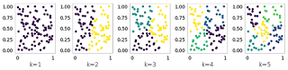
We have previously seen how to implement K-Means. However, the results of this algorithm strongly rely on the choice of the parameter K. In this post, we will see how to use Gap Statistics to pick K in an optimal way. The main idea of the methodology is to compare the clusters inertia on the data to cluster and a reference dataset. The optimal choice of K is given by k for which the gap between the two results is maximum. To illustrate this idea, let’s pick as reference dataset a uniformly distributed set of points and see the result of K-Means increasing K: 

import numpy as np
import matplotlib.pyplot as plt

from sklearn.datasets import make_blobs
from sklearn.metrics import pairwise_distances
from sklearn.cluster import KMeans


reference = np.random.rand(100, 2)
plt.figure(figsize=(12, 3))
for k in range(1,6):
    kmeans = KMeans(n_clusters=k)
    a = kmeans.fit_predict(reference)
    plt.subplot(1,5,k)
    plt.scatter(reference[:, 0], reference[:, 1], c=a)
    plt.xlabel('k='+str(k))
plt.tight_layout()
plt.show()