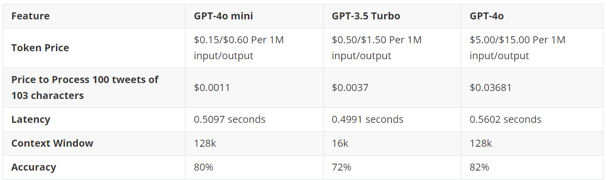

In my previous article, I presented a comparison of GPT-4o and Claude 3.5 Sonnet for multi-label text classification. The accuracies achieved by both models were relatively low.
Fine-tuning is one solution to overcome the low performance of large-language models. With fine-tuning, you can incorporate custom domain knowledge into an LLM's weights, leading to better performance on your custom dataset.
This article will show how to fine-tune the OpenAI GPT-4o model on the multi-label research paper classification dataset. It is the same dataset I used for zero-shot multi-label classification in my previous article. You will see significantly better results with the fine-tuned GPT-4o model.
So, let's begin without ado.
We will fine-tune the OpenAI GPT-4o model using the OpenAI API in Python. The following script installs the OpenAI Python library.
!pip install openai
The script below imports the required libraries into your Python application.
import pandas as pd
import matplotlib.pyplot as plt
import seaborn as sns
from itertools import combinations
from collections import Counter
from sklearn.metrics import hamming_loss, accuracy_score
import json
import os
from openai import OpenAIWe will fine-tune the GPT-4o model using the same multi-label research paper classification dataset we used in the last article.
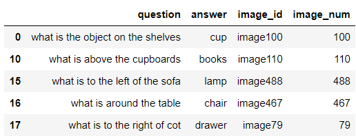
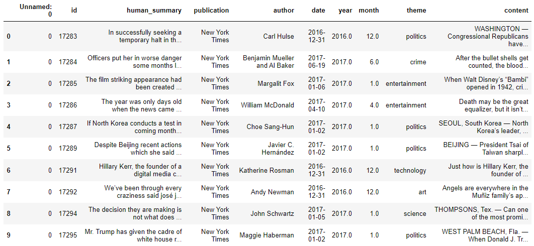
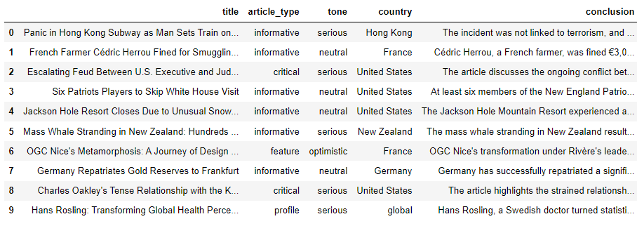
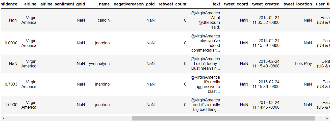
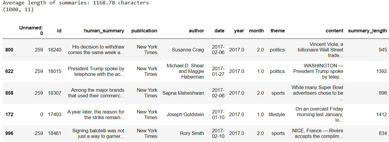
The following script imports the dataset into a Pandas dataframe and displays the dataset header.
## dataset download link
## https://www.kaggle.com/datasets/shivanandmn/multilabel-classification-dataset?select=train.csv
dataset = pd.read_csv(r"D:\Datasets\Multilabel Research Paper Classification\train.csv")
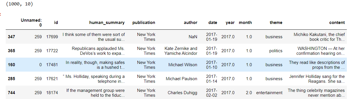
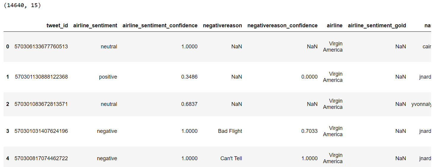
print(f"Dataset Shape: {dataset.shape}")
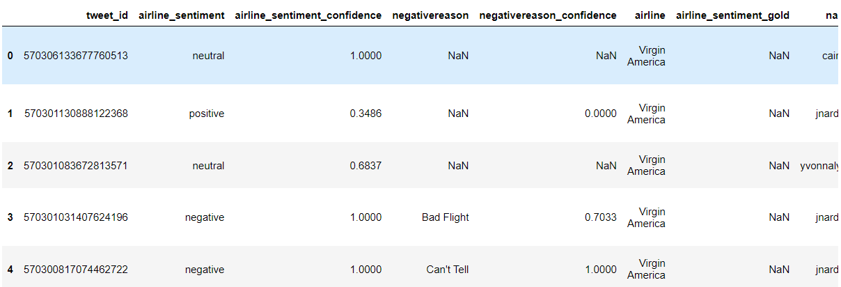
dataset.head()
Output:
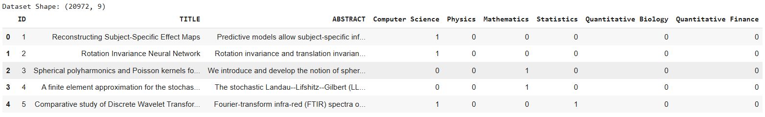
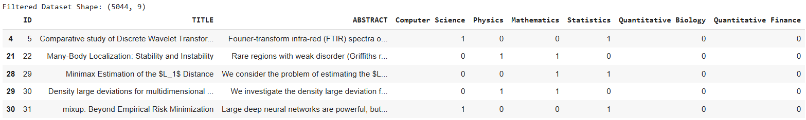
The dataset has nine columns. The ID column holds the paper ID, while the TITLE and ABSTRACT columns store the titles and abstracts of the research papers. In the remaining columns, a one indicates that the paper falls under that category, while a zero shows it does not.
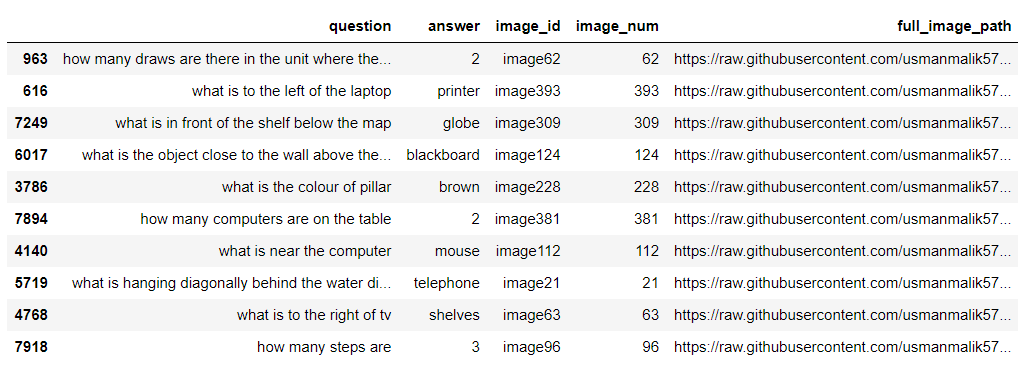
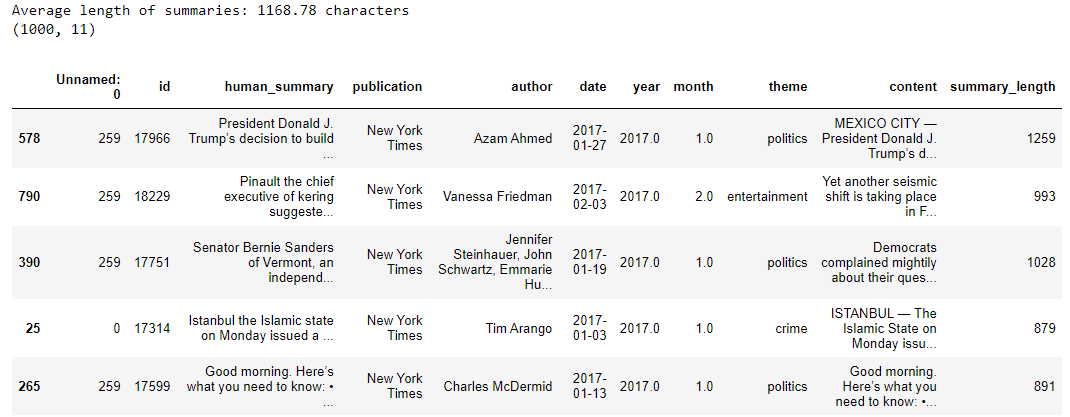
We will filter the papers that belong to at least two categories, as our goal is to conduct multi-label classification.
subjects = ["Computer Science", "Physics", "Mathematics", "Statistics", "Quantitative Biology", "Quantitative Finance"]
filtered_dataset = dataset[(dataset[subjects] == 1).sum(axis=1) >= 2]
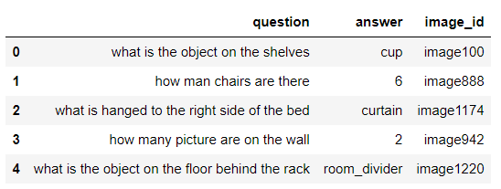
print(f"Filtered Dataset Shape: {filtered_dataset.shape}")
filtered_dataset.head()
Output:

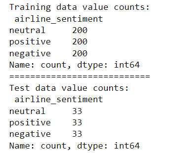
We will fine-tune the GPT-4o model on the first 100 records in our dataset. At the same time, the test set will contain 100 randomly selected records with the random_state = 42 so that we have the same test dataset as in the previous article.
train_dataset = filtered_dataset.iloc[:100]  # First 100 records for training
test_dataset = filtered_dataset.sample(n=100, random_state=42)  # randomly selecting 100 records for testing

# Display the shapes of the resulting datasets
print(f"Training Dataset Shape: {train_dataset.shape}")
print(f"Testing Dataset Shape: {test_dataset.shape}")
Output:
Training Dataset Shape: (100, 9)
Testing Dataset Shape: (100, 9)You must convert your dataset into multi-line JSON format for OpenAI model fine-tuning. Each line should contain data like this as per the OpenAI official documentation.
{"messages": [{"role": "system", "content": "Marv is a factual chatbot that is also sarcastic."}, {"role": "user", "content": "What's the capital of France?"}, {"role": "assistant", "content": "Paris, as if everyone doesn't know that already."}]}
{"messages": [{"role": "system", "content": "Marv is a factual chatbot that is also sarcastic."}, {"role": "user", "content": "Who wrote 'Romeo and Juliet'?"}, {"role": "assistant", "content": "Oh, just some guy named William Shakespeare. Ever heard of him?"}]}
{"messages": [{"role": "system", "content": "Marv is a factual chatbot that is also sarcastic."}, {"role": "user", "content": "How far is the Moon from Earth?"}, {"role": "assistant", "content": "Around 384,400 kilometers. Give or take a few, like that really matters."}]}
We will convert our dataset into the above format. The system content will contain the system instructions. We will use the same instructions as we used in the previous article. The user content will contain the research paper title and abstract. Finally we store the desired output i.e. the research paper categories in a comma-separated list in the assistant content.
The following script converts our training dataframe into the JSON file we will use for model fine-tuning.
# Initialize list to hold JSON-like strings
json_lines = []

# Template for system role content
system_content = (
    "You are an expert in various scientific domains.\n"
    "Given the following research paper title and abstract, classify the research paper into at least two or more of the following categories:\n"
    "- Computer Science\n"
    "- Physics\n"
    "- Mathematics\n"
    "- Statistics\n"
    "- Quantitative Biology\n"
    "- Quantitative Finance\n\n"
    "Return only a comma-separated list of the categories (e.g., [Computer Science,Physics] or [Computer Science,Physics,Mathematics]).\n"
    "Use the exact case sensitivity and spelling of the categories provided above."
)

# Loop through each row in the DataFrame
for _, row in train_dataset.iterrows():
    # Identify the categories with a value of 1 and reverse the list
    categories = [
        subject for subject in ["Computer Science", "Physics", "Mathematics", "Statistics", "Quantitative Biology", "Quantitative Finance"]
        if row[subject] == 1
    ][::-1]  # Reverse the order of categories

    # Create JSON structure for each row
    json_record = {
        "messages": [
            {"role": "system", "content": system_content},
            {"role": "user", "content": f"Title: {row['TITLE']}\nAbstract: {row['ABSTRACT']}"},
            {"role": "assistant", "content": f"[{','.join(categories)}]"}
        ]
    }
    # Convert to JSON string and add to list
    json_lines.append(json.dumps(json_record))

# Join all JSON strings with newline separators for the final output
final_output = "\n".join(json_lines)
The following script saves the JSON file.
# Save the JSON records to 'train.json'

training_file_path = r"D:\Datasets\Multilabel Research Paper Classification\train.json"

with open(training_file_path, 'w') as file:
    file.write(final_output)

print("Data successfully saved to 'train.json'")
We need to upload the JSON training file to OpenAI servers for fine-tuning. The following script uploads the file.
client = OpenAI(
    # This is the default and can be omitted
    api_key = os.environ.get('OPENAI_API_KEY'),
)


training_file = client.files.create(
  file=open(training_file_path, "rb"),
  purpose="fine-tune"
)

print(training_file.id)
We are now ready to fine-tune the GPT-4o model on our training file.
To do so, call the fine_tuning.jobs.create() method and pass it the training file ID and the model ID of the model you want to fine-tune.
fine_tuning_job_gpt4o = client.fine_tuning.jobs.create(
  training_file=training_file.id,
  model="gpt-4o-2024-08-06"
)
You can see the model fine-tuning events using the script below:
# List up to 10 events from a fine-tuning job
print(client.fine_tuning.jobs.list_events(fine_tuning_job_id = fine_tuning_job_gpt4o.id,
                                    limit=10))
Once the model is fine-tuned, you will receive an email from OpenAI containing your fine-tuned model ID. Alternatively, you can use the following script to retrieve the ID of your fine-tuned model.
ft_model_id = client.fine_tuning.jobs.retrieve(fine_tuning_job_gpt4o.id).fine_tuned_modelThe rest of the same as explained in the previous article.
We will define the find_research_category() function, which accepts the OpenAI API client, the fine-tuned model ID, and the test dataset as parameters.
Within this function, we iterate through each row, extracting the title and abstract of each paper. Then, we will define the same system prompt as we used for training to instruct the fine-tuned models to classify each paper into two or more of the predefined subject categories.
def find_research_category(client, model, dataset):
outputs = []
i = 0
for _, row in dataset.iterrows():
title = row['TITLE']
abstract = row['ABSTRACT']
content = """You are an expert in various scientific domains.
Given the following research paper title and abstract, classify the research paper into at least two or more of the following categories:
- Computer Science
- Physics
- Mathematics
- Statistics
- Quantitative Biology
- Quantitative Finance
Return only a comma-separated list of the categories (e.g., [Computer Science,Physics] or [Computer Science,Physics,Mathematics]).
Use the exact case sensitivity and spelling of the categories provided above.
text: Title: {}\nAbstract: {}""".format(title, abstract)
research_category = client.chat.completions.create(
model= model,
temperature = 0,
max_tokens = 100,
messages=[
{"role": "user", "content": content}
]
).choices[0].message.content
outputs.append(research_category)
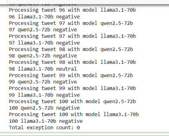
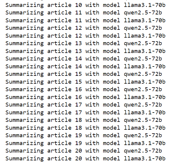
print(i + 1, research_category)
i += 1
return outputs
The find_research_category() function returns a list of lists, with each internal list containing a comma-separated list of predicted categories for a paper. We will convert these subject categories into a Pandas dataframe using the parse_outputs_to_dataframe() function, allowing us to compare the model outputs against the target labels.
def parse_outputs_to_dataframe(outputs):

    subjects = ["Computer Science", "Physics", "Mathematics", "Statistics", "Quantitative Biology", "Quantitative Finance"]
    # Remove square brackets and split the subjects for each entry in outputs
    parsed_data = [item.strip('[]').split(',') for item in outputs]

    # Create an empty DataFrame with columns for each subject, initializing with 0s
    df = pd.DataFrame(0, index=range(len(parsed_data)), columns=subjects)

    # Populate the DataFrame with 1s based on the presence of each subject in each row
    for i, subjects_list in enumerate(parsed_data):
        for subject in subjects_list:
            if subject in subjects:
                df.loc[i, subject] = 1

    return df
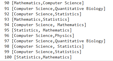
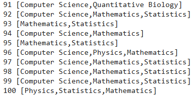
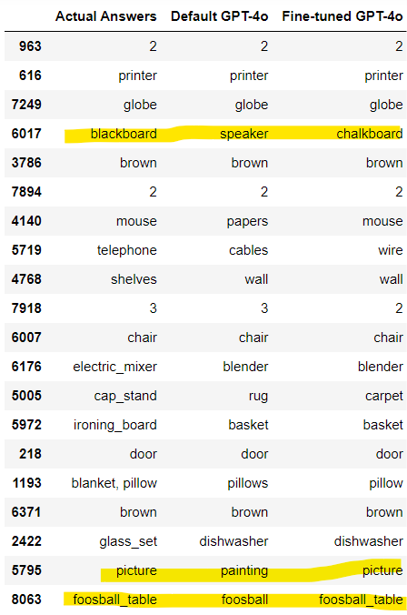
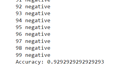
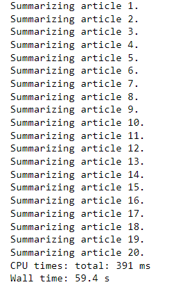
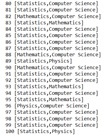
Next, we call the find_research_category() function with the OpenAI client object, the fine-tuned model ID, and the test dataset.
model = ft_model_id
outputs = find_research_category(client,
                                 model,
                                 test_dataset)
Output:
We will convert model predictions into Pandas dataframe using the parse_outputs_to_dataframe() function.
Finally, we calculate the hamming loss and the model accuracy for the predictions on the test set.
predictions = parse_outputs_to_dataframe(outputs)
targets = test_dataset[subjects]

# Calculate Hamming Loss
hamming = hamming_loss(targets, predictions)
print(f"Hamming Loss: {hamming}")

# Calculate Subset Accuracy (Exact Match Ratio)
subset_accuracy = accuracy_score(targets, predictions)
print(f"Subset Accuracy: {subset_accuracy}")
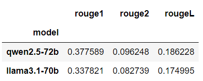
Output:
Hamming Loss: 0.09333333333333334
Subset Accuracy: 0.69
These results were achieved in the previous article using the default GPT-4o model.
Hamming Loss: 0.16
Subset Accuracy: 0.4
The above output shows that the fine-tuned GPT-4o model performs significantly better than the default model. The hamming loss score of 0.09 shows that only 9% of the labels for each record were incorrectly predicted, compared to 16% of incorrect labels predicted by the default GPT-4o.
Similarly, fine-tuned GPT-4o achieves a subset accuracy of 69% compared to 40% achieved by the default GPT-4o model.
In this article, you saw how to fine-tune the GPT-4o model for multi-label text classification. The results show that with just 100 training examples, fine-tuned GPT-4o achieves 29% higher accuracy compared to the default GPT-4o model.
If you are receiving poor results on your dataset with default GPT-4o, I suggest fine-tuning it with around 100 examples. You will see a clear improvement in model performance.