Day: June 16, 2024

As a data scientist, I have extensively used the Hugging Face library for processing unstructured data such as images, text, and audio. My previous blogs have covered various transformer models for these types of data. Lately, however, I discovered that Hugging Face also provides transformer models for tabular data. One such transformer is the Meta Tree Transformer.

This article will explore using the Meta Tree Transformer model to classify tabular data, detailing each process step and providing insights based on the Bank Note Authentication dataset.

You must install and import the following libraries to run the codes in this article.

!pip install metatreelib
!pip install --upgrade scikit-learn
!pip install imodels

from metatree.model_metatree import LlamaForMetaTree as MetaTree
from metatree.decision_tree_class import DecisionTree, DecisionTreeForest
from metatree.run_train import preprocess_dimension_patch
from transformers import AutoConfig
from sklearn.metrics import accuracy_score
import imodels # pip install imodels
import sklearn
from sklearn.model_selection import train_test_split
import numpy as np
import pandas as pd
import torch
from torch.utils.data import Dataset, DataLoader
import random

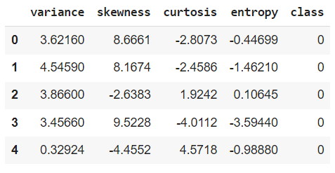
The dataset used in this tutorial is the Bank Note Authentication dataset, which you can download from Kaggle. The dataset contains features extracted from images of banknotes and is used to classify whether a banknote is authentic or not.

The dataset consists of the following columns:

• variance
• skewness
• curtosis
• entropy
• class

The class column is the target variable, indicating whether the banknote is authentic (1) or not (0).

First, we need to read the dataset and preprocess it. We will use the pandas library to read the dataset from a CSV file.

This will load the dataset into a pandas DataFrame and display the first few rows to get an overview of the data.

# Load the dataset
file_path = '/content/BankNote_Authentication.csv'  # Path to the dataset
df = pd.read_csv(file_path)

# Display the first few rows of the dataset
df.head()

Output:

Next, we split the dataset into training and testing sets using sklearn.model_selection.train_test_split. Here, 20% of the data is reserved for testing, ensuring we have sufficient data to evaluate the model's performance.

# Split the dataset into features and target variable
X = df.drop(columns=['class'])
y = df['class']

# Split the data into training and testing sets
train_X, test_X, train_y, test_y = train_test_split(X, y, test_size=0.2,

To handle the entire dataset in batches of 256, we will create a custom dataset class and use PyTorch's DataLoader to batch and shuffle the data. The batch size is set to 256 since the Meta Tree transformer expects the data to be in batches of 256 records.

class TabularDataset(Dataset):
    def __init__(self, features, labels):
        self.features = features
        self.labels = labels

    def __len__(self):
        return len(self.features)

    def __getitem__(self, idx):
        feature = self.features[idx]
        label = self.labels[idx]
        return torch.tensor(feature, dtype=torch.float32), torch.tensor(label, dtype=torch.float32)

# Convert data to tensors
train_features = train_X.values
train_labels = torch.nn.functional.one_hot(torch.tensor(train_y.values), num_classes=2).float().numpy()

# Create Dataset
train_dataset = TabularDataset(train_features, train_labels)

# Parameters
batch_size = 256

# Create DataLoader
train_loader = DataLoader(train_dataset, batch_size=batch_size, shuffle=True)

To begin with, we need to initialize the Meta Tree Transformer model and adjust its configuration to match our dataset, particularly the number of features and classes.

The model is configured to handle a different number of features by default. We set config.n_feature to the number of features in our dataset (train_X.shape[1]).

Similarly, the model is configured for a different number of output classes. We set config.n_class to the number of classes in our dataset (2).

# Initialize Model
model_name_or_path = "yzhuang/MetaTree"

config = AutoConfig.from_pretrained(model_name_or_path)
# Override config parameters to match your dataset
config.n_feature = train_X.shape[1]
config.n_class = 2

model = MetaTree.from_pretrained(
    model_name_or_path,
    config=config,
    ignore_mismatched_sizes=True
)

decision_tree_forest = DecisionTreeForest()

# Set the depth of the model
model.depth = 2

Next, we train the model using the batches provided by the DataLoader.

# Training loop
for batch_features, batch_labels in train_loader:
    # Prepare the batch for the model
    batch = {"input_x": batch_features, "input_y": batch_labels, "input_y_clean": batch_labels}
    batch = preprocess_dimension_patch(batch, n_feature=train_X.shape[1], n_class=2)

    # Generate decision tree
    outputs = model.generate_decision_tree(batch['input_x'], batch['input_y'], depth=model.depth)
    decision_tree_forest.add_tree(DecisionTree(auto_dims=outputs.metatree_dimensions, auto_thresholds=outputs.tentative_splits, input_x=batch['input_x'], input_y=batch['input_y'], depth=model.depth))

    print("Decision Tree Features: ", [x.argmax(dim=-1) for x in outputs.metatree_dimensions])
    print("Decision Tree Thresholds: ", outputs.tentative_splits)

Finally, we evaluate the model's performance on the test set.

# Predict using the decision tree forest
test_X_tensor = torch.tensor(test_X.values, dtype=torch.float32)
tree_pred = decision_tree_forest.predict(test_X_tensor)

tree_pred = tree_pred.argmax(dim=-1).squeeze().numpy()

# Calculate accuracy
accuracy = accuracy_score(test_y, tree_pred)
print("MetaTree Test Accuracy: ", accuracy)

Output:

MetaTree Test Accuracy:  0.8727272727272727

The Meta Tree Transformer offers a powerful method for classifying tabular data by combining the interpretability of decision trees with the robust performance of transformer models. In this tutorial, we walked through the process of setting up the model, preprocessing the data, training with multiple batches, and evaluation.

In my experience, the performance of the Meta Tree Transformer was on par with simpler algorithms like Random Forest and AdaBoost. Experimenting with different parameters and datasets can further enhance its performance, making it a valuable addition to any data scientist's toolkit.

Feel free to leave your feedback and the results you obtained using Transformer models on tabular data.